I came in contact with Asymmetric Numeral Systems first one year ago, when i looked deeper into entropy coding. Whilst stumbling over huffman coders and arithmetic coding, i crossed roads with ANS. At first glance it is surprising, how with those two old coders, which basicly solved entropy coding, such a new development took place. Delving deeper into all those coders, it becomes easy to notice the shortcomings of the two old coders and the elegance of ANS. The industry supports this view, by including ANS in Zstandard, LZFSE, CRAM and many more. Unterstanding ANS at its full took me quite a while (and propably i am still not done with the process). So let me take you along the journey i took and hopefully make unterstanding ANS a little easier.

Some prerequisites

For everyone, who isnt that familar the fundamentals of information theory and entropy coding, lets talk some fundamentals. The core concept of information theory is to send as much information through a bandwith limited chanel as possible. But what is information? Information is a combination of any number of different symbols with meaning to two parties. The sender and the reciever. Now to quantify information, we need to make some definitions. We call the sender source and the source emits symbols \(s\) from an Alphabet \(A\) with properbilites for each symbol \(p_s\). All those properbilites add to one. To keep it simple, we are going to assume, that the probabilites are independent from any previously emitted symbols. Some short dependencies can be fitted in this pattern, by defining a sequence as a unique symbol.

Seeing that each symbol needs to have some sort of informative value, it can be assumed, that this value soly depends on the propability, with which it is emitted. Now we say, that the more frequently a symbol it transimitted, the less suprising it becomes to the reciever, so its informational value is less then a symbol, that is seldomly emitted. Finaly we need a unit, to meassure the information and for that we take bits. Coming from this, the information of a symbol is:

\[I_s = \operatorname{ld}(p_s)\]

With that we can define, how much Information a source emitts on average with every symbol by calculating the weighted average, which is called entropy of a source:

\[H = \sum p_s * I_s\]

Knowig this, we can cleary understand the goal of entropy coding. The output of the entropy encoder should match the information output of the source. The average output of the encoder will be refered to as bitrate \(R\). Now we can meassure the difference of the bitrate and entropy and called that coding redundancy \(\Delta R = R-H\). So by minimizing the coding redundancy we can optimize the entropy coder. As far as the concept of information theory goes, the entropy marks the low bound for the encoder. So any further compression will lead to a loss of information.

One way, to achieve minimum coding redundacy is to give every symbol of the alphabet a codeword, aka a bitsequence, of variable length, matching the information of the symbol. Assuming all propabilities would be roughly similar, that would lead to equal length codewords, which is real easy and wont require any complex fiddling with entropy coding. So we only want to use data, with extrem symbol distributions. Giving each symbol a codeword of variable length matching its information is exactly, what huffman coding does. But by doing this, we will run into a few core issues. First, the minimum encodable information is one bit. So if we have a symbol with less information, we loose bandwith. This continues, as we are limitied to full bit information values, whereas real data doesnt follow these propabilited, again introducing a loss of bandwith and therby creating a necessity for new coders. Enter ANS

ANS

To make ANS really simple, we take a state \(x\) and a symbol \(s\) and create a state machine that turns those two into a new state \(x'\). For decoding the new state must be created in a way, that it reliably returns the old state \(x\) and the encoded symbol \(s\). Further more for optimal encoding, the bitrepresentation of the new state needs to be the same size as the sum of the bit representation of the old state and the information of the symbol. One super simple example of this principle would be simulating a binary source emitting symbols with the same frequency and calling the symbols \([0,1]\). So each symbol has a propability of 0.5 and thereby \(I=\operatorname{ld}{0.5}=1bit\). So we have to symbols and want to spend on bit on encoding each symbol. Now encoding means turning a binary sequence, aka the binary representation of a number into a decimal and decoding doing the reverse. Now we want to perform this operation sequentially, so we wont run into any issues for encoding very long messages or sources that emmit symbols over a period of time. This gives us the encoding and decoding functions:

\[C(x,s) = x*2+s\] \[s = x\operatorname{mod} 2\] \[D(x) = \left\lfloor \frac{x}{2}\right\rfloor\]

As we see, the encoding function takes a state and a symbol and returns a new state. The decoding function reverses the operation of the encoding function and takes a state and returns a new state and a decoded symbol. This example could now be furter customized to suit different symbol distributions, describing uABS furter. But for general purpose the more general approach for broader examples is range ANS, which will be disscused next.

rANS

The previous example was only capable to encode alphabets with two symbols. This is a rare usecase, as most sources at least use an 8 bit or even 32 bit symbolspace. Furthermore a more general approach for encoding with variable symbolpropablilites is needed. For those reasons we have range ANS (rANS). The idea of rANS remains the same, to have a simple state transition machine. Now we just need to define a formula, that fullfills our condition for optimal coding. One more thing, that would be really practial, would be, if the formula was real easy to compute. So, we should preferebly skip complex divisions, floatingpoint operations and very big numbers. But currently the propabilites are floating point values, so lets change that and turn them into frequencies. This can be done relatviley precisly, but that is a point where we are at risk of loosing precision. Further more lets say, that all frequencies have to add up to something that is describalble by \(2^n, n \in \mathbb{N}\), aka, let the sum be a power of two. The importence of this will become obvious in a moment. Now lets call the frequency of a symbol \(L_s\) and the sum \(\sum{L_s} = L\). Now the frequency of a symbol will be considered a range, a number of slots of states for decoding and the all the appended ranges can be considered a block. These blocks repeat infinitly, until the message is encoded. To make this a bit more graphical, lets look at an example:

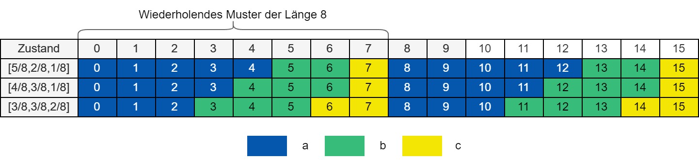
What we can see here is repeating blocks of the size eight with varying ranges for different symboldistributions. Now we can take a closer look at one of these distributions and an encoding example:

Okay, so whats happening in this example. First we see, that we have a Source with the following properties: \(A = [a,b,c],\, L=8, L_a=5,\,L_b=2,\,L_c=1\). Furhtermore the initial state \(x_0 = 0\) and we are in the proccess of encoding “aba”. The first row has all the possible states, which are like array indices. The next three rows have their own ongoing indices, but only in their ranges. Encoding works now by searching the current state in the range indices of the symbol. This index is now the new state which sumarizes the encoded symbol and old state. One issue becomes already obvious in this example: Lets say we want to encode “aaaa”, which would, beginning at an initial state of 0, lead to the final state of 0. Decoding “aaa” would result in the same state. If we change the initial state from 0 to anything else we are safe from this behaviour. Furthermore it turns out, that encoding an infrequent symbol like c leads to much bigger state changes then encoding a frequent symbol. Now lets turn this into a computable formula. So we need again a forumula that turns a state and a symbol into a new state. The new state is determined by three factors. First we need to identify the new block, then the range inside of the block and finally the exact position inside the range. For decoding this happens with:

\[C(x_{t+1},s)=\left\lfloor\frac{x_t}{L_s}\right\rfloor \cdot L+ \mathrm{CDF}[s] + x_t\operatorname{mod} L_s.\]

Now lets take a close look, at what does what. First of all \(\left\lfloor\frac{x_t}{L_s}\right\rfloor\) identifies the blockindex. But since we count in states, we need to multiply the blockindex by the length of each block. Next we need to find the range. This happens by finding the first state in a block, which is reachable by writing a symbol s. In our example the first position for writing a b would be 5 and for writing a c would be 7. As these values stay the same for all blocks they can be precomputed by simply calculating the cummulative distribution function. For the example it looks like this: \(CDF = [a:0,b:5,c:7]\). To make it even easier, we can turn the symbols into numbers and have them directily be the index inside the CDF. Last \(x_t\operatorname{mod} L_s\) ensures, that the next state remains inside the allowed range. And that is rANS in a nutstell. Decoding works exactly in reveresed order. First we need to find the symbol. For that we create a symbols table, which looks like this: symbols = [a,a,a,a,a,b,b,c]. So now we can divide the state by L and the reminder is the index of the symbol inside the symbols table.

\[x_t = D(s,x_{t+1})=L_s \cdot \left\lfloor\frac{x_{t+1}}{L}\right\rfloor - \mathrm{CDF}[s]+x_{t+1}\operatorname{mod} L \, \text{ with } \, s = \mathrm{symbol}\left[x_{t+1}\operatorname{mod} L\right]\]

Decoding works by backtracking every single step we took in encoding. As I found the formualas quite confusing when first checking out ANS, lets see how this works in practice:

\(x_1= C(x_0,b)=\left\lfloor\frac{x_0}{L_b}\right\rfloor \cdot L + \mathrm{CDF}[b] + x_0\mod L_b = \left\lfloor\frac{8}{2}\right\rfloor \cdot 8 + 5 + 8\mod 2 = 37\) \(x_2=C(x_1,s_a)=\left\lfloor\frac{x_1}{L_a}\right\rfloor \cdot L+ \mathrm{CDF}[a] + x_1\mod L_a = \left\lfloor\frac{37}{5}\right\rfloor \cdot 8 + 0 + 37\mod 5 = 58\) \(x_3=C(x_2,s_a)=\left\lfloor\frac{x_2}{L_a}\right\rfloor \cdot L+ \mathrm{CDF}[a] + x_2\mod L_a = \left\lfloor\frac{58}{5}\right\rfloor \cdot 8 + 0 + 58\mod 5 = 91\) \(x_4=C(x_3,s_a)=\left\lfloor\frac{x_3}{L_c}\right\rfloor \cdot L+ \mathrm{CDF}[c] + x_3\mod L_c = \left\lfloor\frac{91}{1}\right\rfloor \cdot 8 + 7 + 91\mod 1 = 735\)

and lets decode the state again:

\(s_4 = \mathrm{symbol}\left(735\mod 8\right) = \mathrm{symbol}(7) = c\) \(x_3 = D(x_4)=L_c \cdot \left\lfloor\frac{x_4}{L}\right\rfloor - \mathrm{CDF}[c]+x_4 \mod L = 1 \cdot \left\lfloor\frac{735}{8}\right\rfloor - 7+735\mod 8 = 91\) \(s_3 = \mathrm{symbol}\left(91\mod 8\right) = \mathrm{symbol}(3) = a\) \(x_2 = D(x_3)=L_a \cdot \left\lfloor\frac{x_3}{L}\right\rfloor - \mathrm{CDF}[a]+x_3\mod L = 5 \cdot \left\lfloor\frac{91}{8}\right\rfloor - 0+91\mod 8 = 58\) \(s_2 = \mathrm{symbol}\left(58\mod 8\right) = \mathrm{symbol}(2) = a\) \(x_1 = D(x_4)=L_a \cdot \left\lfloor\frac{x_2}{L}\right\rfloor - \mathrm{CDF}[a]+x_2\mod L = 5 \cdot \left\lfloor\frac{58}{8}\right\rfloor - 0+58\mod 8 = 37\) \(s_1 = \mathrm{symbol}\left(37\mod 8\right) = \mathrm{symbol}(7) = b\) \(x_0 = D(x_4)=L_b \cdot \left\lfloor\frac{x_1}{L}\right\rfloor - \mathrm{CDF}[b]+x_1\mod L = 2 \cdot \left\lfloor\frac{37}{8}\right\rfloor - 7+37\mod 8 = 8\)

Now that the purly mechanical part is hopefully a bit clearer, lets look at some optimations. First we said, we want L to be a power of two and no complex divisions. But here we have quite a few divisions and modulo operations. With l being a power of two we can turn modulo and division in faster bitshift and bitlogic operations:

\[x_t = L_s \cdot (x_{t+1} >> m) - \mathrm{CDF}[s]+x_{t+1} \& (L-1) \, \text{ mit } \, s = \mathrm{symbol}\left[x_{t+1} \& (L-1)\right]\]

L now turns into \(2^m\). This is also a good point to discuss the meaning of m and thereby the size of L. First, L has to be greater then the amount of symbols in our alphabet, because the smallest frequency a symbol can have is one. Secondly, the size of L limits the precission, with which we can code the symbol-propablilites. Lets say, we have a symbol, that occures with \(p_s = 0.001\), the first good approximation happens at \(L=1024\) and \(L_s = 1\). Any smaller L would force us to encode the symbol with a wrong frequency and thereby with too much or too little information. That’s why m is called preccisionbits, becuase m controls the amount of precision we give to our coder. Now you might say, allright, if few precisionbits hurt the coding, lets just make it very big. But this leads to new issues, which brings us to the most important point of this whole topic. Does it even work and if yes, how well?

To answer this question, lets take a closer look at the coding function. The coding function consists of three parts which are added together. For \(\mathrm{CDF}[s]\) and \(x_t\operatorname{mod} L_s\) we can define a constant upper limit. The limit for the CDF is L, as that is the sum of all frequencies. Now lets think about the upper limit for the second term. Say, we only code one symbol, forcing \(L_s = L\). So the upper limit of this is also L. This means with every coding step we add in the worst case \(2L\) to the state. The bigger the state gets, the smaller the influece of this constant and limited part gets. So we only need to proof, that \(x_{new} = \left\lfloor\frac{x}{L_s}\right\rfloor \cdot L\) works optimal. For that lets look at a more formal defintion of optimality. We say, that the bits requiered to display a state should be the sum of Information of all the encoded symbols to get to that state, which is described by:

\[\operatorname{ld}(x_new) = \operatorname{ld}(x) + \operatorname{ld}(\frac{1}{p_s})\]

Now the propablity is \(L/L_s\), resulting in:

\[\operatorname{ld}(x_new) = \operatorname{ld}(x) + \operatorname{ld}(\frac{L}{L_s})\]

This can be turned into:

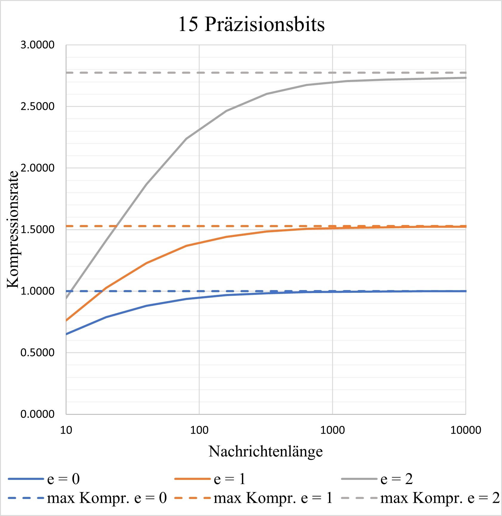
\[x_new = \frac{x}{L_s} * L\]

which is exactly, what we use for encoding. Hereby we have a proof, that ANS is somewhat optimal. Now lets take a closer look at the influence of the constant part on the optimality. The smaller the state is, the more bits are required to encorporate the overhead of the encoding function. The greater the state gets, the less additional bits are required for the overhead. To get a better understanding of this, I ran a small test. The test is already over a year old and was used for a uni project. Because of that the image description is currently in german. This will be changed in the future. For the test i created a random source emitting symbols with very uneven propabilities. Next i calculated the theoretical max compression ratio. A ratio of 2 would equal cutting the bits needed for the message in half. Then i created a load of random messages from the source with different lengths and calculated the average compression ratio. The results show, that for very short messages we even end up with an expansion. Coming close to 1000 symols we reach allmost optimal coding. For future research i also want to take a look at what different alphabetsizes and different amounts of precision bits do to the optimality.

On this thaught i like to end my first chapter to ANS and hope, i could help you understand the core concept on ANS a bit better.

---