<?xml version="1.0" encoding="utf-8"?><feed xmlns="http://www.w3.org/2005/Atom" ><generator uri="https://jekyllrb.com/" version="3.10.0">Jekyll</generator><link href="https://hanusspi.github.io/feed.xml" rel="self" type="application/atom+xml" /><link href="https://hanusspi.github.io/" rel="alternate" type="text/html" /><updated>2026-07-24T19:43:15+00:00</updated><id>https://hanusspi.github.io/feed.xml</id><title type="html">Hans Nusspickel</title><subtitle>Computer Science Student | Graphics &amp; Simulation Enthusiast</subtitle><author><name>Hans Nusspickel</name></author><entry><title type="html">Neighborhood Search for Particle Systems</title><link href="https://hanusspi.github.io/2025/09/27/SpatialHasing.html" rel="alternate" type="text/html" title="Neighborhood Search for Particle Systems" /><published>2025-09-27T00:00:00+00:00</published><updated>2025-09-27T00:00:00+00:00</updated><id>https://hanusspi.github.io/2025/09/27/SpatialHasing</id><content type="html" xml:base="https://hanusspi.github.io/2025/09/27/SpatialHasing.html"><![CDATA[<h1 id="1-introduction">1. Introduction</h1>
<p>In the previous posts, we looked a lot into fluid simulation. One major aspect of fluid simulation is the neighborhood search. Previously we just glanced over the fact and solved the issue using a library. Today we want to explore one method in more detail to achieve a faster neighborhood search.</p>

<h1 id="2-neighborhood-search">2. Neighborhood Search</h1>
<p>For simplicity, let’s say we want to create a simple particle simulation, where we spawn a bunch of particles in the beginning and just run collision detection between the particles and a bounding box.</p>

<p>First we need to detect collisions, which will be the main focus. Then later on we will talk about the collision resolution. From our collision we need two major pieces of information. How deep is the collision, so how big is the overlap and in which direction. So for particles, the direction is the difference of center coordinates of both particles.</p>

<p>Checking if a particle collides with an AABB (axis aligned bounding box) is easy, by comparing the x,y,z coordinates to the x,y,z coordinates of the two points defining the AABB. Therefore we just iterate over all particles, compare if the particle center is closer than the particle radius to the boundary and apply forces accordingly to resolve the collision.</p>

<p>The more complicated part is, finding inter particle collisions. First lets define the distance between two spheres a and b:
\(d = ||p_1 - p_2|| - (r_1 + r_2).\)
If the distance is smaller than 0, we have a collision, and already the value we need for resolution.</p>

<p>So one way to check, would be to simply compare all sphere positions to each other:</p>

<figure class="highlight"><pre><code class="language-text" data-lang="text"><table class="rouge-table"><tbody><tr><td class="gutter gl"><pre class="lineno">1
2
3
4
5
6
7
8
9
10
11
12
13
14
</pre></td><td class="code"><pre>FOR (size_t i = 0; i &lt; particles.size(); ++i) {
    FOR (size_t j = i + 1; j &lt; particles.size(); ++j) {
        glm::vec3 direction = particles[j].position - particles[i].position;
        float distance = glm::length(direction);
        float minDistance = particles[i].radius + particles[j].radius;

        if (distance &lt; minDistance) {
            float overlap = minDistance - distance;
            CollisionPair collision{
                i, j, overlap, glm::normalize(direction)
            };
            collisions.push_back(collision);
        }
    }
</pre></td></tr></tbody></table></code></pre></figure>

<p>Since we have two nested for loops both with length <code class="language-plaintext highlighter-rouge">particles.size()</code> we have a runtime of \(O(n^2)\) with n being the number of particles. For 100 particles this might be still ok, but for 1.000 particles we already need to run 1.000.000 comparisons and for 10.000 particles 100.000.000 comparisons. Considering that our basic fluid simulations ran with 20.000 particles already, we need to find a faster solution.</p>

<h1 id="3-spatial-hashing">3. Spatial Hashing</h1>
<p>A major component of accelerating the search is the use of spatial acceleration data structures. For one we could add a voxel grid to our domain with a voxel size of the particle radius. Now we denote which particle lives in which voxel cell. If we now want to know which particles might have a collision with particle a, we simply in 2D look at the cell that particle a is in and the 8 surrounding cells. For the 3D case we then have to search 27 cells. Therefore for each particle we have to only look at a fixed amount of cells. This approach is considered a dense grid representation. Let’s take a look at an example:</p>

<figure style="text-align: center;">
  <img src="\img\posts\2025-09-27-SpatialHashing\HashingDenseGrid.png" alt="Sparse Hash Grid" style="max-width: 80%;" />
  <figcaption style="font-style: italic; color: #666; margin-top: 5px;">Dense Hash Grid</figcaption>
  </figure>

<p>Logically this means that first we iterate over all particles, determine each particle’s cell id and increment the count of particles for each cell. The cell id is the index in the cell array. For later access we then create an entry points array. At the index i, the entry points array tells us at which index in the particle array we have to look for the particles of the cells. And at the index i + 1 of the entry points array we get the index of the next starting particle for the next cell (and thereby the index of the last element as the predecessor).</p>

<p>Performing the neighborhood search now is easy, by determining the indices of the neighboring 26 cells, looking up the particles inside the cells and iterating over them.</p>

<p>This approach has a few issues though. First it forces us to determine the domain size in the beginning, which limits the dynamic evolution of the scene. Second, most simulations have a high air to particle ratio, rendering many cells empty. And lastly, by design this approach works best if there is only a small amount of particles in a cell. Therefore the cells should be small. All factors combined can lead to very big grids with very few entries, being slow and memory hungry.</p>

<p>To circumvent this, instead of calculating our index like in the marching cubes example, we introduce a hash function:</p>

\[hash(coords) = |((coords.x * 73856093) ^ (coords.y * 19349663) ^ (coords.z * 83492791))| \mod numCells\]

<p>First of all, now we can also see negative indices, since an integer coordinate is simply the world coordinate divided by the cell size. Therefore we need to force the result into a positive range. Next we can preselect how many cells we want to have. Choosing too many cells leads to many sparse entries. Choosing too few cells can lead to overlap. Two different integer coordinates can lead to the same index. To minimize this, literature suggests using large prime numbers. If the overlap is not too big, we will simply iterate over a few more entries.</p>

<figure style="text-align: center;">
  <img src="\img\posts\2025-09-27-SpatialHashing\HashingSparse.png" alt="Dense Hash Grid" style="max-width: 80%;" />
  <figcaption style="font-style: italic; color: #666; margin-top: 5px;">Dense Hash Grid</figcaption>
  </figure>

<p>Therefore the general process is very similar. One thing we didn’t look at yet is how to determine the particle array and how to actually build the entry points array. The second image shows a simple way of creating the particle array, by first building up a partial sums array that simply adds up as the entries continue over the index. Next we fill in each particle into the particle array, with the index being determined by the subsequent partial sums entry and decrement the entry in the partial sums array. This leaves us with a particle array and a partial sums array.</p>

<p>Dependent on how often the neighborhood information needs to be accessed, the neighborhood information can also be cached in a neighbors array, as done in my code sample <a href="https://github.com/hanusspi/BasicParticleSimulation">https://github.com/hanusspi/BasicParticleSimulation</a>.</p>

<p>Considering that this implementation is very poorly optimized and majorly created as a test bed for a bigger framework, we can still see drastic performance improvements growing with the number of particles. And most importantly, doubling the number of particles only halves instead of quarters the framerate now.</p>

<h1 id="4-summary">4. Summary</h1>

<p>Today we analyzed one major bottleneck in particle based simulations and derived two new methods of improving the performance. Firstly we built up an easier system using dense grid spatial data structure and then improved performance even further by applying sparse hash grids. While this helps performance a lot, especially the fluid simulation still runs very slow, as it is highly serialized. One means to improve performance would be to increase clock rates of the CPU. But here we are very limited. And if we cannot scale in depth, we have to scale in width. While CPUs are still very limited in this department, GPUs are not. Therefore next time we will take a deeper look at leveraging GPUs to gain massive performance improvements.</p>]]></content><author><name>Hans Nusspickel</name></author><summary type="html"><![CDATA[1. Introduction In the previous posts, we looked a lot into fluid simulation. One major aspect of fluid simulation is the neighborhood search. Previously we just glanced over the fact and solved the issue using a library. Today we want to explore one method in more detail to achieve a faster neighborhood search.]]></summary></entry><entry><title type="html">Turning Particles into a Fluid</title><link href="https://hanusspi.github.io/2025/09/25/Meshgeneration.html" rel="alternate" type="text/html" title="Turning Particles into a Fluid" /><published>2025-09-25T00:00:00+00:00</published><updated>2025-09-25T00:00:00+00:00</updated><id>https://hanusspi.github.io/2025/09/25/Meshgeneration</id><content type="html" xml:base="https://hanusspi.github.io/2025/09/25/Meshgeneration.html"><![CDATA[<h1 id="1-introduction">1. Introduction</h1>
<p>In the last post we created our first pressure solver and got some pretty good results. Real fluids though do not really look like a bunch of spheres, but have a closed fluid surface. To resolve this issue, we define a function that can tell us how far a point in space is from the fluid surface. To do this we will define a signed distance function, that works with the lagrangian fluid simulation. Furthermore we need a strategy to create points, for which we can sample the distance to the surface and turn those points into a grid. And this is what we will start with.</p>

<h1 id="2-marching-cubes">2. Marching Cubes</h1>
<p>To start off with marching cubes algorighm [LC87] we overlay the simulation domain with a voxel grid. The length of a voxel we will denote with \(l\). Next we sample some function, in most cases a signed distance field (sdf) \(\Phi\) at each corner point \(x_i\) of each voxel.</p>

<iframe srcdoc="&lt;!DOCTYPE html&gt;
&lt;html lang=&quot;en&quot;&gt;
&lt;head&gt;
    &lt;meta charset=&quot;UTF-8&quot;&gt;
    &lt;meta name=&quot;viewport&quot; content=&quot;width=device-width, initial-scale=1.0&quot;&gt;
    &lt;title&gt;Marching Squares Animation&lt;/title&gt;
    &lt;style&gt;
        body {
            margin: 0;
            padding: 20px;
            background: white;
            color: black;
            font-family: &quot;Courier New&quot;, monospace;
            display: flex;
            flex-direction: column;
            align-items: center;
        }

        canvas {
            border: 2px solid #ccc;
            background: white;
            border-radius: 8px;
        }

        .controls {
            margin: 20px;
            display: flex;
            gap: 10px;
        }

        button {
            padding: 10px 20px;
            background: #e94560;
            color: white;
            border: none;
            border-radius: 5px;
            cursor: pointer;
            font-family: inherit;
        }

        button:hover {
            background: #c73650;
        }

        .info {
            max-width: 600px;
            text-align: center;
            margin: 20px;
            line-height: 1.6;
        }

        .step-info {
            background: #f0f0f0;
            padding: 15px;
            border-radius: 8px;
            margin: 10px 0;
            min-height: 50px;
            border: 1px solid #ddd;
        }
    &lt;/style&gt;
&lt;/head&gt;
&lt;body&gt;
    &lt;h1&gt;Marching Squares Algorithm&lt;/h1&gt;

    &lt;canvas id=&quot;canvas&quot; width=&quot;600&quot; height=&quot;600&quot;&gt;&lt;/canvas&gt;

    &lt;div class=&quot;controls&quot;&gt;
        &lt;button onclick=&quot;startAnimation()&quot;&gt;Start Animation&lt;/button&gt;
        &lt;button onclick=&quot;stepForward()&quot;&gt;Next Step&lt;/button&gt;
        &lt;button onclick=&quot;stepBackward()&quot;&gt;Previous Step&lt;/button&gt;
        &lt;button onclick=&quot;reset()&quot;&gt;Reset&lt;/button&gt;
    &lt;/div&gt;

    &lt;div class=&quot;step-info&quot; id=&quot;stepInfo&quot;&gt;
        Click &quot;Start Animation&quot; to see how marching squares works!
    &lt;/div&gt;

    &lt;div class=&quot;info&quot;&gt;
        &lt;p&gt;This animation shows the marching squares algorithm step by step:&lt;/p&gt;
        &lt;p&gt;1. First, we define a shape using a Signed Distance Function (SDF)&lt;br&gt;
        2. We overlay a grid and sample the SDF at each grid point&lt;br&gt;
        3. We find where the surface crosses grid edges (where SDF changes sign)&lt;br&gt;
        4. Finally, we connect these crossing points to form the contour&lt;/p&gt;
    &lt;/div&gt;

    &lt;script&gt;
        const canvas = document.getElementById(&quot;canvas&quot;);
        const ctx = canvas.getContext(&quot;2d&quot;);
        const stepInfo = document.getElementById(&quot;stepInfo&quot;);

        const width = canvas.width;
        const height = canvas.height;
        const gridSize = 40;
        const centerX = width / 2;
        const centerY = height / 2;
        const sphereRadius = 180;

        let animationStep = 0;
        let animationFrame = null;
        let isAnimating = false;

        // Simple sphere SDF
        function sphereSDF(x, y) {
            const dx = x - centerX;
            const dy = y - centerY;
            const distFromCenter = Math.sqrt(dx * dx + dy * dy);
            return distFromCenter - sphereRadius; // negative inside, positive outside
        }

        function interpolate(p1, p2, v1, v2) {
            if (Math.abs(v1 - v2) &lt; 0.001) return p1;
            const t = -v1 / (v2 - v1);
            return {
                x: p1.x + t * (p2.x - p1.x),
                y: p1.y + t * (p2.y - p1.y)
            };
        }

        function drawBackground() {
            ctx.fillStyle = &quot;white&quot;;
            ctx.fillRect(0, 0, width, height);
        }

        function drawSphere() {
            ctx.save();
            ctx.globalAlpha = 0.2;

            // Draw filled circle
            ctx.beginPath();
            ctx.arc(centerX, centerY, sphereRadius, 0, Math.PI * 2);
            ctx.fillStyle = &quot;#4a90e2&quot;;
            ctx.fill();

            ctx.restore();
        }

        function drawGrid() {
            ctx.strokeStyle = &quot;#ccc&quot;;
            ctx.lineWidth = 1;

            // Vertical lines
            for (let x = gridSize; x &lt; width; x += gridSize) {
                ctx.beginPath();
                ctx.moveTo(x, 0);
                ctx.lineTo(x, height);
                ctx.stroke();
            }

            // Horizontal lines
            for (let y = gridSize; y &lt; height; y += gridSize) {
                ctx.beginPath();
                ctx.moveTo(0, y);
                ctx.lineTo(width, y);
                ctx.stroke();
            }
        }

        function drawSDFValues() {
            ctx.font = &quot;12px Courier New&quot;;
            ctx.textAlign = &quot;center&quot;;

            for (let x = 0; x &lt;= width; x += gridSize) {
                for (let y = 0; y &lt;= height; y += gridSize) {
                    const sdf = sphereSDF(x, y);
                    const isInside = sdf &lt; 0;

                    // Draw point
                    ctx.beginPath();
                    ctx.arc(x, y, 4, 0, Math.PI * 2);
                    ctx.fillStyle = isInside ? &quot;#e94560&quot; : &quot;#4a90e2&quot;;
                    ctx.fill();

                    // Draw value
                    ctx.fillStyle = isInside ? &quot;#c73650&quot; : &quot;#2c5aa0&quot;;
                    ctx.fillText(sdf.toFixed(0), x, y - 8);
                }
            }
        }

        function drawInterpolatedPoints() {
            const points = [];

            for (let x = 0; x &lt; width; x += gridSize) {
                for (let y = 0; y &lt; height; y += gridSize) {
                    if (x + gridSize &lt;= width &amp;&amp; y + gridSize &lt;= height) {
                        const corners = [
                            {x: x, y: y, sdf: sphereSDF(x, y)},
                            {x: x + gridSize, y: y, sdf: sphereSDF(x + gridSize, y)},
                            {x: x + gridSize, y: y + gridSize, sdf: sphereSDF(x + gridSize, y + gridSize)},
                            {x: x, y: y + gridSize, sdf: sphereSDF(x, y + gridSize)}
                        ];

                        // Check each edge for zero crossings
                        for (let i = 0; i &lt; 4; i++) {
                            const c1 = corners[i];
                            const c2 = corners[(i + 1) % 4];

                            if ((c1.sdf &lt; 0) !== (c2.sdf &lt; 0)) {
                                const point = interpolate(
                                    {x: c1.x, y: c1.y},
                                    {x: c2.x, y: c2.y},
                                    c1.sdf, c2.sdf
                                );
                                points.push(point);
                            }
                        }
                    }
                }
            }

            // Draw interpolated points
            ctx.fillStyle = &quot;#ff8800&quot;;
            points.forEach(point =&gt; {
                ctx.beginPath();
                ctx.arc(point.x, point.y, 6, 0, Math.PI * 2);
                ctx.fill();
            });
        }

        function drawContour() {
            ctx.strokeStyle = &quot;#00aa44&quot;;
            ctx.lineWidth = 3;

            for (let x = 0; x &lt; width; x += gridSize) {
                for (let y = 0; y &lt; height; y += gridSize) {
                    if (x + gridSize &lt;= width &amp;&amp; y + gridSize &lt;= height) {
                        const corners = [
                            {x: x, y: y, sdf: sphereSDF(x, y)},
                            {x: x + gridSize, y: y, sdf: sphereSDF(x + gridSize, y)},
                            {x: x + gridSize, y: y + gridSize, sdf: sphereSDF(x + gridSize, y + gridSize)},
                            {x: x, y: y + gridSize, sdf: sphereSDF(x, y + gridSize)}
                        ];

                        const intersections = [];

                        // Find intersections on edges
                        for (let i = 0; i &lt; 4; i++) {
                            const c1 = corners[i];
                            const c2 = corners[(i + 1) % 4];

                            if ((c1.sdf &lt; 0) !== (c2.sdf &lt; 0)) {
                                const point = interpolate(
                                    {x: c1.x, y: c1.y},
                                    {x: c2.x, y: c2.y},
                                    c1.sdf, c2.sdf
                                );
                                intersections.push(point);
                            }
                        }

                        // Draw line between intersections
                        if (intersections.length &gt;= 2) {
                            ctx.beginPath();
                            ctx.moveTo(intersections[0].x, intersections[0].y);
                            ctx.lineTo(intersections[1].x, intersections[1].y);
                            ctx.stroke();
                        }
                    }
                }
            }
        }

        function drawStep() {
            drawBackground();

            switch (animationStep) {
                case 0:
                    stepInfo.textContent = &quot;Step 1: Show the shape (sphere) we want to trace&quot;;
                    drawSphere();
                    break;

                case 1:
                    stepInfo.textContent = &quot;Step 2: Overlay a grid&quot;;
                    drawSphere();
                    drawGrid();
                    break;

                case 2:
                    stepInfo.textContent = &quot;Step 3: Sample SDF at grid points (red = inside, blue = outside)&quot;;
                    drawSphere();
                    drawGrid();
                    drawSDFValues();
                    break;

                case 3:
                    stepInfo.textContent = &quot;Step 4: Find interpolated points where surface crosses edges (orange dots)&quot;;
                    drawGrid();
                    drawSDFValues();
                    drawInterpolatedPoints();
                    break;

                case 4:
                    stepInfo.textContent = &quot;Step 5: Connect crossing points to form the final contour!&quot;;
                    drawGrid();
                    drawSDFValues();
                    drawInterpolatedPoints();
                    drawContour();
                    break;
            }
        }

        function animate() {
            if (!isAnimating) return;

            drawStep();

            if (animationStep &lt; 4) {
                setTimeout(() =&gt; {
                    animationStep++;
                    animate();
                }, animationStep === 0 ? 2000 : animationStep &lt; 2 ? 2000 : 3000);
            } else {
                isAnimating = false;
            }
        }

        function startAnimation() {
            animationStep = 0;
            isAnimating = true;
            animate();
        }

        function stepForward() {
            isAnimating = false;
            if (animationStep &lt; 4) {
                animationStep++;
            }
            drawStep();
        }

        function stepBackward() {
            isAnimating = false;
            if (animationStep &gt; 0) {
                animationStep--;
            }
            drawStep();
        }

        function reset() {
            animationStep = 0;
            isAnimating = false;
            drawBackground();
            stepInfo.textContent = &quot;Click \&quot;Start Animation\&quot; to see how marching squares works! Or use \&quot;Next Step\&quot; for manual control.&quot;;
        }

        // Initialize
        reset();
    &lt;/script&gt;
&lt;/body&gt;
&lt;/html&gt;" width="100%" height="800" frameborder="0"></iframe>

<p>The first major issue of this algorithm is indexing. We have a 3d voxel grid, but need to store everything in a 1d array. Therefore we determine unique integer coordinates (i,j,k) (which are easy to translate into world space) with (0,0,0) at the origin of the grid. Given the size of our simulation domain, which we can represent as an Axis Aligned Bounding Box (AABB) we can determine how many voxel cells the grid has in each dimension, denoted by \(n_x, n_y, n_z\). Next we need to map each integer coordinate to a vertex (corner of a voxel) with</p>

<p>\(V = in_y n_z + j n_z + k\).</p>

<p>In the same fashion a cell can be identified with</p>

<p>\(C = in_y n_z + j n_z + k\).</p>

<p>Even though we have one less cell in each direction than vertices. But for simplicity we keep it like that.</p>

<p>And lastly we need a function to define edges</p>

\[E = 3 V + dir,\]

<p>where dir is 0,1,2 for x,y,z.</p>

<p>For the full implementation we will have to handle some literal edge cases, because vertices on the outer side of the grid do not have edges in all directions.</p>

<p>The nice thing about those functions is, that they are bijective, therefore from a vertex id we can backtrack to its integer and finally world coordinates. Given the world coordinate x we can sample \(\phi(x)\) and get for the vertex i \(\Phi_i = \Phi(x_i)\).</p>

<p>With this information we know if a vertex is inside or outside of the surface. This already gives us some basic information, but not a mesh yet.</p>

<p>Therefore next we will iterate over all edges and check if they intersect the surface, i.e. if the sign between the vertices making up the edge changes. If we have a sign change, we calculate an edge weight by linear interpolation giving us the intersection point. This gives us a solid guess of where the actual surface could be. It is important that we store these points in relation to the edge they belong to. Since our surface is going to have a lot fewer points than we have voxels, it is sensible to store them in a map.</p>

<figure style="text-align: center;">
  <img src="/img/posts/2025-09-25-Meshgeneration/MarchingCubesEdit.svg.png" alt="Marching Cubes visualization" style="max-width: 80%;" />
  <figcaption style="font-style: italic; color: #666; margin-top: 5px;">Source: Wikipedia</figcaption>
  </figure>

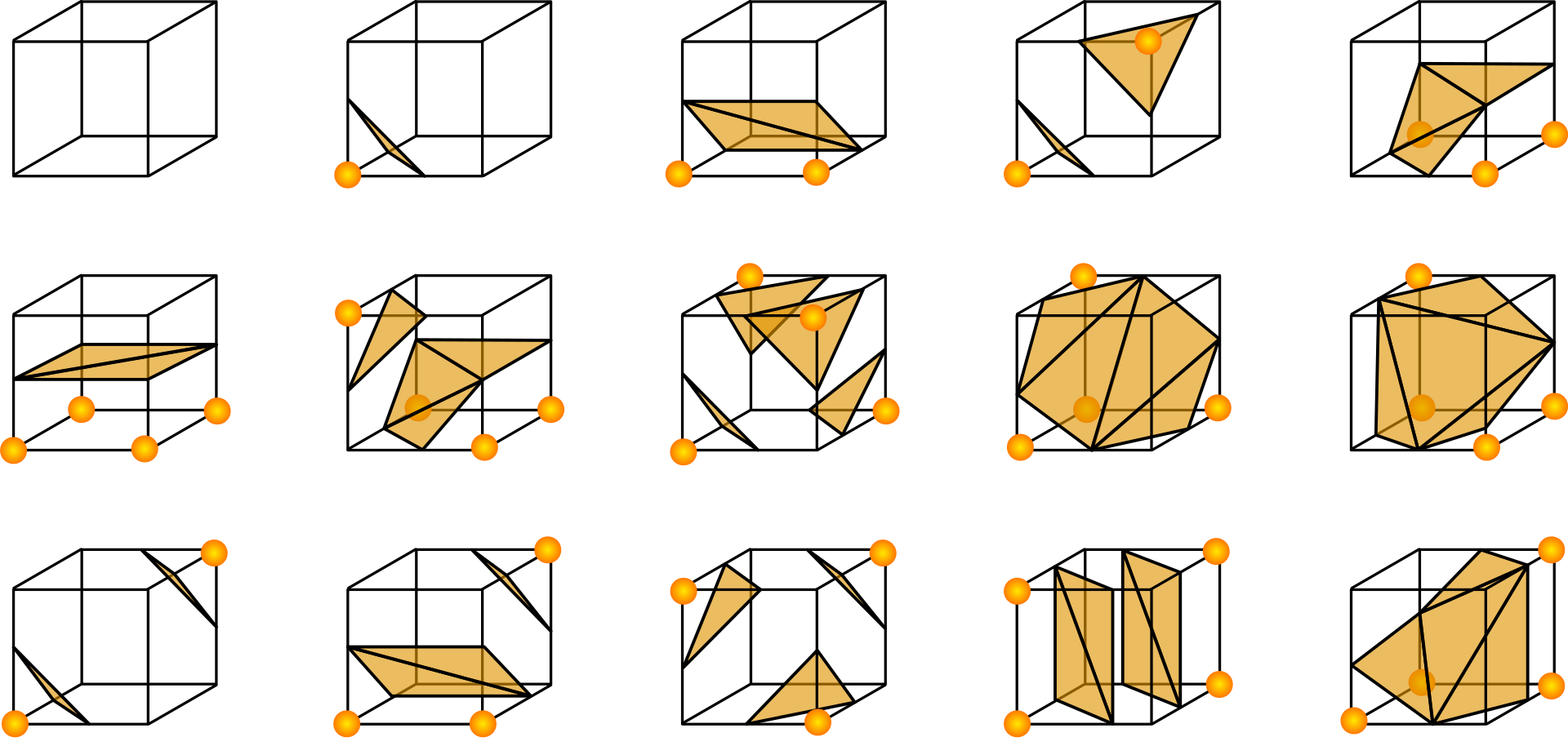
<p>In the last step we need to append the vertex data with geometric connectivity. For this a marching cubes table exists, that we can use. As visible in the image above, the marching cube table tells us, based on which edges experiencing a sign change, which vertices to connect. And for this to work properly, all the previous hassle with indexing was required.</p>

<p>Lastly, to get a smooth mesh, we do not just need to have vertices and connectivity, but also vertex normals. These we can either calculate in the beginning for the voxel corners and interpolate later on or calculate in a second sweep for the exact vertex positions.</p>

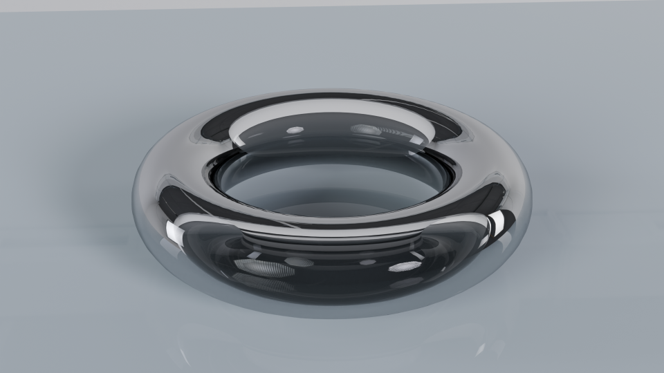
<p>Applying this for an object with a known signed distance function, like a torus yields this result:</p>

<figure style="text-align: center;">
<img src="/img/posts/2025-09-25-Meshgeneration/torus.png" alt="Torus generated using marching cubes" style="max-width: 80%;" />
<figcaption style="font-style: italic; color: #666; margin-top: 5px;">Torus mesh generated using the marching cubes algorithm</figcaption>
</figure>

<h1 id="3-fluid-surface-reconstruction">3. Fluid Surface Reconstruction</h1>

<p>To make marching cubes work we therefore need a \(\Phi\) that we can sample. While for primitive shapes, like a torus, sphere or square these are analytically defined, for our fluid they are not. Therefore we need a function that is close to 1, if it is inside the fluid and 0 or even negative if it is outside of the fluid. Applying some fundamentals of the SPH idea and using the method how we determine the value of quantites in SPH (as discusses in the last posts) gives us [BJ25]</p>

\[\Phi(\mathbf{x})=-c+\sum_{j\in\mathcal{N}(\mathbf{x})}\frac{1}{\rho_j}W(\mathbf{x}-\mathbf{x}_j,h),\]

<p>where \(\rho_j\) is now the normalized density estimation</p>

\[\rho_i=\sum_{j\in\mathcal{N}(\mathbf{x}_i)}W(\mathbf{x}_i-\mathbf{x}_j,h).\]

<p>We are required to add a slightly negative c to force a sign change, since the second part of the function will never get smaller than 0. By choosing the c we can determine how tight or loose we want the surface to be. A good starting value is 0.55.</p>

<p>Since this formulation seemingly requires a neighborhood search, it seems to be pretty expensive. Since unlike the particles, our vertices are grid aligned and indexable though, we can turn things around and iterate over the particles, determine an AABB around each particle, check which vertices are in the interior of the AABB and then write the values to the vertices. The only disadvantage of this approach is that it is very hard to parallelize.</p>

<p>In the very beginning we defined the cell size as a parameter. We want to set the cell size so that a sole particle can create a single mesh, to prevent particles suddenly popping up and vanishing later on. Therefore a good cell size is 1.0 times the particle radius.</p>

<h1 id="4-results">4. Results</h1>

<p>Applying marching cubes and the newly defined sdf gives us this lovely result for our previously generated simulation</p>

<video width="70%" controls="">
  <source src="/img/posts/2025-09-25-Meshgeneration/DamBreak.mp4" type="video/mp4" />
  Your browser does not support the video tag.
</video>

<p>Depending on the rendering settings in Blender the look of the fluid can be varied even further.</p>

<h1 id="5-summary">5. Summary</h1>
<p>In this post we started out by defining a voxel grid with many indices turning it into the marching cube algorithm [LC87]. Finally we managed to apply it to a particle based fluid simulation turning it into a real fluid.
The code can be found under <a href="https://github.com/hanusspi/BasicPressureSolverLab">https://github.com/hanusspi/BasicPressureSolverLab</a>, where the mesh gets generated as a vtk and can be imported into blender using the same workflow as for the particles in the previous blog post.</p>

<h1 id="references">References</h1>

<p>[LC87] W.E. Lorensen and H.E. Cline. Marching cubes: A high resolution 3d surface construction algorithm. ACM Computer Graphics, 21(4):163–169, 1987.
[BJ25] Prof. Dr. Jan Bender, M.Sc. Timna B¨ottcher, M.Sc. Jos´e Fern´andez, M.Sc. Lukas Westhofen: Fluid Simulation in Computer Graphics</p>]]></content><author><name>Hans Nusspickel</name></author><summary type="html"><![CDATA[1. Introduction In the last post we created our first pressure solver and got some pretty good results. Real fluids though do not really look like a bunch of spheres, but have a closed fluid surface. To resolve this issue, we define a function that can tell us how far a point in space is from the fluid surface. To do this we will define a signed distance function, that works with the lagrangian fluid simulation. Furthermore we need a strategy to create points, for which we can sample the distance to the surface and turn those points into a grid. And this is what we will start with.]]></summary></entry><entry><title type="html">Our first SPH Solver</title><link href="https://hanusspi.github.io/2025/06/14/FirstPressureSolver.html" rel="alternate" type="text/html" title="Our first SPH Solver" /><published>2025-06-14T00:00:00+00:00</published><updated>2025-06-14T00:00:00+00:00</updated><id>https://hanusspi.github.io/2025/06/14/FirstPressureSolver</id><content type="html" xml:base="https://hanusspi.github.io/2025/06/14/FirstPressureSolver.html"><![CDATA[<h1 id="1-introduction">1. Introduction</h1>

<p>In the previous chapters I talked alot about physics and maths building up some fundamental ideas of why and how the lagrangian viewpoint can  be applied to fluid simulation. Now it is time, to turn the formulas into an algorithm and code to start some fluid simulation. The algorightms we use to simulate fluid, are generally called pressure solvers, since that is exactly what they do.</p>

<h1 id="2-wcsph">2. WCSPH</h1>

<p>There is many ways to implement an SPH Solver, but one of the oldest and simplest (and easiest to understand) is Weakly Compressible SPH.</p>

<p>Let me start by showing you the general algorithm and then jump into the details and some practically relevant side notes.</p>

<figure class="highlight"><pre><code class="language-text" data-lang="text"><table class="rouge-table"><tbody><tr><td class="gutter gl"><pre class="lineno">1
2
3
4
5
6
7
8
9
10
11
12
13
14
15
16
17
18
19
</pre></td><td class="code"><pre>// SPH (Smoothed Particle Hydrodynamics) Algorithm

FOR each particle i:
    find_neighbors(i) → neighbors_j

FOR each particle i:
    density_i = SUM(mass_j * kernel_weight(i,j)) for all neighbors j
    pressure_i = state_equation(density_i)

FOR each particle i:
    pressure_acceleration_i = -(1/density_i) * gradient(pressure_i)
    viscosity_acceleration_i = viscosity * laplacian(velocity_i)
    other_acceleration_i = gravity
    
    total_acceleration_i = pressure_force_i + viscosity_force_i + other_force_i

FOR each particle i:
    velocity_i(t + dt) = velocity_i(t) + dt * total_force_i 
    position_i(t + dt) = position_i(t) + dt * velocity_i(t + dt)
</pre></td></tr></tbody></table></code></pre></figure>

<p>The first step is the neighborhood search. For starters we will be using CompactNSearch to do this for us. This offers a relatively well optimized, fast and accesible way to do the neighborhood search.</p>

<p>In the next step we need to see, how the current situation looks. Therefore we compute the density for all fluid particles including boundaries as we have discussed in the last post. Finally we can apply the EOS (equation of state) to determine the pressure for each particle.</p>

<p>Knowing the pressure, we can now determine a resulting force. The force is dependent the particle mass, which is static, the density, which we just calculated and the gradient of the pressure.</p>

\[\mathbf{F}_i^p = -\frac{m_i}{\rho_i} \nabla p_i \approx -\underbrace{\sum_{j \in N_i^f} m_j \left(\frac{p_i}{\rho_i^2} + \frac{p_j}{\rho_j^2}\right) \nabla W_{ij}}_{\text{fluid-fluid interaction}} - \underbrace{\sum_{k \in N_i^b} \rho_0 V_k \frac{p_i}{\rho_i^2} \nabla W_{ik}}_{\text{fluid-solid interaction}}\]

<p>Here we can see the use of the altered derivative to ensure symmetric forces between particles. Dividing the pressure force by the particles mass then gives us an acceleration:</p>

\[\mathbf{a}_i^p = \mathbf{F}_i^p / m_i\]

<p>Combine this with the acceleration due to viscosity:</p>

\[\mathbf{a}_i^v = \nu \nabla^2 \mathbf{v}_i \approx 2\nu_f \sum_{j \in N_i^f} \frac{m_j}{\rho_j} (\mathbf{v}_i - \mathbf{v}_j) \frac{(\mathbf{x}_i - \mathbf{x}_j)^T \nabla W_{ij}}{|\mathbf{x}_i - \mathbf{x}_j|^2 + 0.01h^2} + 2\nu_b \sum_{k \in N_i^b} V_k \mathbf{v}_i \frac{(\mathbf{x}_i - \mathbf{x}_k)^T \nabla W_{ik}}{|\mathbf{x}_i - \mathbf{x}_k|^2 + 0.01h^2}\]

<p>And applying gravity gives us all the resulting accelerations for our particle.</p>

<p>In the final step we apply the accleration using the Semi Implicit Euler method to update the velocity and finally the position.</p>

<h1 id="3-discusstion-and-specialties">3. Discusstion and Specialties</h1>

<p>Having looked at the general proccess it is easier to explain the name. What we are doing is looking at the current situation and based on that we derive an update. But we do not know, if the update will improve the situation. After all we could push many particles into one area creating a new pressure hot spot. This use of an explicit solving method makes the weackly compressible in the name.</p>

<p>To minimze the error we make by doing this, we have to select a very small timestep size. Which size exactly always depends on the dynamics of the simulation and all other parameters. A second factor that limits our timestep size is the boundary handling method. Currently we have a single layer of boundary particles that the fluid particle should never cross or it will be gone for ever. To express and calculate this limitation, we use the CFL-Condition:</p>

\[\Delta t_{CFL} \leq 0.5 \frac{r}{||\mathbf{v}_{max}||}\]

<p>Which we can either use to determine a dynamic timestep size by looking at the fastest particle or which we can use to limit the particle velocities for a fixed timestep size.</p>

<p>In the previous post we also discussed (at least a bit) an extra model for cohesiona and adhesion. This model gives us forces, that we can simply add to the other Forces in the algorithm and include it that way.</p>

<p>Lastly we need to discuss an issue with the equation of state. Currently we simply derive a pressure from the density deviation. Furthermore we simulate a single phase liquid, therefore we are not having any surrounding air particles or something like this. This means, that especially on the surface and in splashes we will see negative pressures. These pressures would suck up other fluid particles and build clumps. While this might sound like surface tension, it is a very much unwanted and bad looking effect. Therefore we simply modify our EOS: \(p_i = \max(0, \kappa (\rho_i - \rho_0))\) to ignore negative pressures and only handle postive pressures.</p>

<h1 id="4-turning-it-into-code">4. Turning it into code</h1>

<p>Having an algorithm and having a running simulator are two very different pairs of shoes. Therefore i want to take a few lines to talk about the actual implementation and some potential error sources. The full code for this project is available <a href="https://github.com/hanusspi/BasicPressureSolverLab">here: https://github.com/hanusspi/BasicPressureSolverLab</a></p>

<p>The procect is coded in C++ as most libraries in this domain are available in C++. Furthermore, it offers the best compromise between beeing fast and still readable enough, to be well understood and fast programmed.</p>

<p>First of all, we need to find a way to define boundaries. For this I used the tinyobject loader and object files, which can be created in blender. Next we need a method to sample the particles. Here I got some good code from a class at my Uni. As did I get a few more helping functions. Afther we have loaded our boundary, and populated it with boundary particles, we apply a first neighborhood search and determine the boundary weights and volumes.</p>

<p>Next we need to define our fluid particles. For simplicity we will start out with sampling a cube with a regular grid and make every grid cell corner a particle. While from a readability stand point it might me nicer to create now a struct, that holds all the particles properties, like its mass, density, position and acceleration. But having a vector of structs is fairly slow compared to having a struct of vectors (or just many vectors). Vectors being like lists, not the mathematical thing.</p>

<p>In the next step we can implement a simulation loop that and update our particle positions. Sadly we do not really have any way of seeing the results right now. Of course there are many ways, for visualizaation, like adding a graphics api and showing the results directly.</p>

<p>One thing you will note though, the simulation runs very slow. Therefore for now we will simply export the particles into .vtk files. That is file format originally created for paraview, but also useable in blender using: .</p>

<p>Now we can run our simulation, drink a cup of coffee, maybe have full meal (or two) and then we will look at the results.</p>

<h1 id="5-results">5. Results</h1>

<p>After 5 minutes we can look at the first results of the breaking dam scene. For this we spawn a grid of particles and advect them according to the pressure solver. For starters we set the viscosity very low. As particle diameter we choose 0.005m and we run the simulation with 3000Hz. This means for one second of footage we need to run the neighborhood search 3000 times. In future we will explore different solvers that can hopefully run at a lower frequency. This is what makes the computation very slow. As we can see, the particles look like fluid, but non the less, we still have the look of a ball pit and not really the look of water. This issue will be fixed in a future post.</p>
<video width="100%" controls="">
  <source src="/img/posts/2025-06-13-FirstPressureSolver/DamBreak.mp4" type="video/mp4" />
  Your browser does not support the video tag.
</video>

<h1 id="6-summary">6. Summary</h1>

<p>Today we took a big step and implemented the first pressure solver. It still is relativley basic, but it works. Right now we still face to big problems. First, a simulation takes very long, second it does not look like water. Those will be things, that we hopefully can change in the next posts.</p>]]></content><author><name>Hans Nusspickel</name></author><summary type="html"><![CDATA[1. Introduction]]></summary></entry><entry><title type="html">Further SPH Fundamentals</title><link href="https://hanusspi.github.io/2025/06/13/Fluid-Simulation2.html" rel="alternate" type="text/html" title="Further SPH Fundamentals" /><published>2025-06-13T00:00:00+00:00</published><updated>2025-06-13T00:00:00+00:00</updated><id>https://hanusspi.github.io/2025/06/13/Fluid-Simulation2</id><content type="html" xml:base="https://hanusspi.github.io/2025/06/13/Fluid-Simulation2.html"><![CDATA[<h1 id="1-introduction">1. Introduction</h1>

<p>In the last post, we began exploring the fundamentals of SPH Fluid Simulation. First, we introduced the general physical framework of fluid simulation and then began turning it into a more computer-friendly system. But all that we have so far is a fluid-fluid interaction. Therefore, we are now able to spawn some fluid in vacuum and have it behave (not even really realistically). So the next step will be to explore how we can compute some coupling between the fluid and solids. Furthermore, we explored the first part of the Navier-Stokes equation, but have not yet explored viscosity. Last but not least, we will take a quick peek at some more effects that the Navier-Stokes equation does not account for.</p>

<h1 id="2-fluid-solid-coupling">2. Fluid-Solid Coupling</h1>

<p>Since we are representing our fluid as discrete particles that are interacting with each other, the intuitive approach is to simply represent the boundary as particles as well. And exactly that is what we are going to do.</p>

<p>First, we sample the boundary with boundary particles. Those particles need to be treated differently in our simulation, since they are never going to move. Next, we need to determine the weight of the boundary particles. Unlike fluid particles, who get all the same weight, we would have to sample the boundary particles all with perfectly equal distance to be able to do this. Since this is not very practical, we simply apply our kernel function and first determine the implied volume of each boundary particle depending on its neighborhood.</p>

\[V_i = \frac{m}{\rho_i} = \frac{m}{\sum_k m W_{ik}} = \frac{1}{\sum_k W_{ik}}\]

<p>You might see a pattern arise here. Most of fluid simulation works by summing up some kernel function over its neighborhood. The advantage of the volume approach is that it is independent of the mass or density. Now the question is, which density our boundary should have. Maybe one could guess that it depends on the boundary material, but since we only care about the effect on the fluid, we assume they have the rest density of the fluid.</p>

<p>With that in mind, the density of a fluid particle turns into:</p>

\[\rho_i = \sum_j m_j W_{ij} + \rho_0 \sum_k V_k W_{ik}\]

<p>Knowing this, we can apply our previous knowledge for building a fluid simulator.</p>

<h1 id="3-viscosity">3. Viscosity</h1>

<p>Viscosity is defined by a fluid’s rate/dependent resistance to a change in shape or to movement of its neighboring positions relative to one another. At least by Wikipedia…</p>

<p>What this means is that viscosity describes the internal friction between adjacent layers of fluid. Since we are having particles and the particle’s velocity, we can therefore derive something to simulate viscosity:</p>

\[\mathbf{a}_i^v = \nu \nabla^2 \mathbf{v}_i \approx 2\nu_f \sum_{j \in N_i^f} \frac{m_j}{\rho_j} (\mathbf{v}_i - \mathbf{v}_j) \frac{(\mathbf{x}_i - \mathbf{x}_j)^T \nabla W_{ij}}{|\mathbf{x}_i - \mathbf{x}_j|^2 + 0.01h^2} + 2\nu_b \sum_{k \in N_i^b} V_k \mathbf{v}_i \frac{(\mathbf{x}_i - \mathbf{x}_k)^T \nabla W_{ik}}{|\mathbf{x}_i - \mathbf{x}_k|^2 + 0.01h^2}\]

<p>While this looks huge, mean, and complicated, we just need to know a few things. First, we get an acceleration of our fluid particle. The magnitude of the acceleration depends on the velocity difference of the particle relative to its neighbors or boundary (since the boundary doesn’t move, we do not have to subtract anything). Furthermore, we get two parameters. One for the fluid viscosity \(\nu_f\) and one for the boundary viscosity \(\nu_b\) with which we can set up the behavior of our fluid.</p>

<p>While one might argue that especially water is not viscous, we will still apply a small bit of viscosity to ensure numerical stability. This means, by discretization we make a small error every timestep. And this might lead to an increasingly growing error and run away: an explosion (at least visually). And to prevent this behavior, viscosity is a good dampening mechanic.</p>

<h1 id="4-surface-tension-adhesion-and-cohesion">4. Surface Tension (Adhesion and Cohesion)</h1>

<p>Lastly, I want to introduce a simple version of surface tension. If we were to spawn a cube of water in space, in nature the cube would turn into a droplet, since water always strives to minimize its surface area. This is an effect that SPH by default does not recreate. The same effect is also responsible for droplet building on surfaces.</p>

<p>Therefore, we introduce a cohesion force which, by applying a different kernel, strives to minimize the surface area of the fluid. For simplicity, I’ll just link to the authors of the paper and not introduce any new formulas.</p>

<p>Next, we add an adhesion force, which simulates the wetting effect of fluids and the tendency to stick to the boundary.</p>

<p>Taking a look at cohesion, we can see with an increasing cohesion factor we get droplet building.</p>

<video width="100%" controls="">
  <source src="/img/posts/2025-06-13-Fluid-Simulation2/adhesion.mp4" type="video/mp4" />
  Your browser does not support the video tag.
</video>

<h1 id="5-summary">5. Summary</h1>

<p>In this a bit shorter chapter, we collected the final puzzle pieces to start building a first fluid simulator. For that, we first thought of a way to handle boundaries to create interesting simulations. Then we introduced viscosity as a natural dampening factor and added adhesion and cohesion forces to generate a more natural fluid behavior.</p>]]></content><author><name>Hans Nusspickel</name></author><summary type="html"><![CDATA[1. Introduction]]></summary></entry><entry><title type="html">Introduction to SPH fluid simulation</title><link href="https://hanusspi.github.io/2025/06/12/Introduction-to-SPH-fluid-simulation.html" rel="alternate" type="text/html" title="Introduction to SPH fluid simulation" /><published>2025-06-12T00:00:00+00:00</published><updated>2025-06-12T00:00:00+00:00</updated><id>https://hanusspi.github.io/2025/06/12/Introduction-to-SPH-fluid-simulation</id><content type="html" xml:base="https://hanusspi.github.io/2025/06/12/Introduction-to-SPH-fluid-simulation.html"><![CDATA[<script src="https://cdnjs.cloudflare.com/ajax/libs/Chart.js/3.9.1/chart.min.js"></script>

<h1 id="1-introduction-to-fluid-simulation">1. Introduction to Fluid Simulation</h1>

<p>One of the more interesting topics in physics-based animation is the simulation of water and fluids in general. The relevance of this topic reaches from computer games, like Sea of Thieves, where a real-time simulation of the ocean is relevant, over VFX art for movies, like Avatar: The Way of Water, to many industrial applications like casting steel.</p>

<p>While there is a lot of research being done on this topic, I first came into contact with it during a physics-based animations lecture and have since worked hard on getting a deeper insight into the topic. Here I want to begin by introducing the fundamentals and then take a dive into some deeper topics that I am currently interested in.</p>

<p>There exist two (and a half) approaches for fluid simulation: the Lagrangian particle-based one and the Eulerian grid-based one. Furthermore, there is a lot of research going into hybrid models that try to combine the best out of both worlds. For now, I will focus on the Lagrangian approach.</p>

<h1 id="2-navier-stokes-equation">2. Navier-Stokes Equation</h1>

<p>First, let’s think about what characteristics make a fluid a fluid and especially let’s think about water. First, of course, it can flow freely and will always try to find a position of lowest energy. Furthermore, it is not compressible. So, (to an extent) no matter how deep you dive into the ocean, 1 cubic meter of water will always have the same amount of water molecules, no matter how high the pressure is. (Very much unlike air, which is very compressible) Finally, we have some more specific properties like surface tension.</p>

<p>The fundamental aspect of fluid simulation though is maintaining the incompressibility through time. And while this post will have a few formulas, I strive to make it as easy and interesting to understand as possible. And I promise in future posts, things will get more programming-centric. The incompressibility can simply be described by \(\frac{D \rho}{D t} = 0 \Leftrightarrow \nabla \cdot v = 0\). $\rho$ denotes the density. The second part implies the same, but we will not use it any further.</p>

<p>From this we can derive the Navier-Stokes equation:
\(\frac{D\mathbf{v}}{Dt}=-\frac{1}{\rho}\nabla p+\nu\nabla^2\mathbf{v}+\frac{\mathbf{f}}{\rho}\)
First of all, we are describing an acceleration. This acceleration has three components:</p>

<ol>
  <li>
    <p>\(-\frac{1}{\rho}\nabla p\): Acceleration due to pressure differences in the fluid.</p>
  </li>
  <li>
    <p>\(\nu\nabla^2\mathbf{v}\): Acceleration due to friction forces between particles in the fluid. This is generally known as viscosity.</p>
  </li>
  <li>
    <p>\(\frac{\mathbf{f}}{\rho}\): Accelerations due to external forces. The forces are normalized to a unit volume. The major force being used is gravity, but it can also be used to induce waves.</p>
  </li>
</ol>

<h1 id="3-smoothed-particle-hydrodynamics-sph">3. Smoothed Particle Hydrodynamics (SPH)</h1>

<p>Currently, we managed to describe the properties of what we want to simulate with a formula. This is a good beginning, but the formula describes something temporally and spatially continuous, which we cannot compute. Therefore, we introduce a spatial discretization into finitely many particles. These particles are not really particles (but we call them that for simplicity) but more like probes giving us information about important field values like density and velocity at a position. This form of discretization makes it a Lagrangian viewpoint.</p>

<p>Having done the first step, we will use a trick to use this for discretization using the Dirac-Delta Distribution. This distribution has the simple characteristic that it is always zero, except at the point x where it jumps to infinity. Formally this looks like:</p>

\[\delta(x)=\begin{cases}\infty&amp;\mathrm{if~}x=0 \\ 0&amp;\mathrm{otherwise}&amp;\end{cases}\]

\[\int_{-\infty}^{+\infty}\delta(x)dx=1\]

<p>Given a function \(f:\Omega\to\mathbb{R}^n\) that maps a position vector \(x\) in the domain \(\Omega \subset \mathbb{R}^3\) to a scalar or vector value, it can be rewritten using the Dirac delta identity:</p>

\[f(x)=\int_\Omega f(x^*)\delta(x-x^*)dx^*\]

<p>While this does not really help us yet to determine somehow what values/properties our particles have, we can now simply rewrite the Dirac Delta identity using a kernel function.</p>

\[f(\mathbf{x})=\int_\Omega f(\mathbf{x}^*)\delta(\mathbf{x}-\mathbf{x}^*)d\mathbf{x}^*\]

\[\approx\int_{D_{\mathbf{x}}}f(\mathbf{x}^*)W(\mathbf{x}-\mathbf{x}^*,h)d\mathbf{x}^*\]

<p>Our kernel function will have to fulfill a few requirements. As we saw, the Dirac delta identity sums up to 1. This must be the case for the kernel function as well. Furthermore, it needs to be symmetric, positive, and have a compact condition. This simply means that it only returns a positive value as long as we are in a set radius, and otherwise we are just 0. For now, we will use the cubic spline kernel, which looks like this:</p>

\[W(q) = \alpha \begin{cases}
\frac{2}{3} - q^2 + \frac{1}{2}q^3 &amp; \text{if } 0 \leq q &lt; 1 \\
\frac{1}{6}(2-q)^3 &amp; \text{if } 1 \leq q &lt; 2 \\
0 &amp; \text{if } q \geq 2
\end{cases}\]

<p>where \(q = \frac{\|\mathbf{x}_i - \mathbf{x}_j\|}{h}\) and $\alpha$ is the normalization constant depending on in how many dimensions we run the simulation.</p>

<p>Taking a closer look at the relationship between the kernel function and the Dirac Delta identity:</p>

<canvas id="sph-kernels-chart" width="700" height="500"></canvas>
<script>
(function() {
    // Cubic spline kernel (different smoothing lengths)
    function cubicSpline(r, h) {
        const q = Math.abs(r) / h;
        const sigma = 1 / h; // normalization constant (1D)
        
        if (q >= 2) return 0;
        if (q < 1) return sigma * (1 - 1.5 * q * q + 0.75 * q * q * q);
        return sigma * 0.25 * (2 - q) * (2 - q) * (2 - q);
    }
    
    // X values from -2 to 2
    const x = [];
    for (let i = -2; i <= 2; i += 0.02) {
        x.push(i);
    }
    
    // Different kernel smoothing lengths
    const kernels = [
        { h: 0.3, color: 'orange', label: 'h=0.3' },
        { h: 0.5, color: 'lightgreen', label: 'h=0.5' },
        { h: 0.7, color: 'cyan', label: 'h=0.7' },
        { h: 0.9, color: 'blue', label: 'h=0.9' },
        { h: 1.1, color: 'purple', label: 'h=1.1' }
    ];
    
    const datasets = kernels.map(kernel => ({
        label: kernel.label,
        data: x.map(xi => ({ x: xi, y: cubicSpline(xi, kernel.h) })),
        borderColor: kernel.color,
        backgroundColor: 'transparent',
        borderWidth: 3,
        pointRadius: 0,
        tension: 0
    }));
    
    // Add Dirac delta approximation (arrow pointing up)
    datasets.push({
        label: 'δ(x)',
        data: [{ x: 0, y: 0 }, { x: 0, y: 12 }],
        borderColor: 'red',
        backgroundColor: 'transparent',
        borderWidth: 4,
        pointRadius: 0,
        showLine: true
    });
    
    // Add arrowhead for Dirac delta
    datasets.push({
        label: '',
        data: [{ x: -0.05, y: 11.5 }, { x: 0, y: 12 }, { x: 0.05, y: 11.5 }],
        borderColor: 'red',
        backgroundColor: 'red',
        borderWidth: 3,
        pointRadius: 0,
        showLine: true,
        fill: true
    });
    
    const ctx = document.getElementById('sph-kernels-chart').getContext('2d');
    new Chart(ctx, {
        type: 'line',
        data: { datasets },
        options: {
            responsive: true,
            scales: {
                x: {
                    type: 'linear',
                    min: -2,
                    max: 2,
                    ticks: { stepSize: 0.5 },
                    title: { display: true, text: 'Distance (r/h)', font: { size: 14 } }
                },
                y: {
                    min: 0,
                    max: 13,
                    ticks: { stepSize: 2 },
                    title: { display: true, text: 'Kernel Weight W(r,h)', font: { size: 14 } }
                }
            },
            plugins: {
                legend: { 
                    display: true,
                    position: 'top',
                    labels: { filter: function(item) { return item.text !== ''; } }
                },
                title: {
                    display: true,
                    text: 'SPH Cubic Spline Kernels vs Dirac Delta Function',
                    font: { size: 16 }
                }
            }
        }
    });
    
    // Add text annotation for Dirac delta
    setTimeout(() => {
        const canvas = document.getElementById('sph-kernels-chart');
        const ctx = canvas.getContext('2d');
        ctx.fillStyle = 'red';
        ctx.font = '14px Arial';
        ctx.textAlign = 'center';
        ctx.fillText('δ(x)', canvas.width/2, 50);
        ctx.fillText('(h→0)', canvas.width/2, 65);
    }, 100);
})();
</script>

<p>It becomes more obvious to see how an increasingly smaller h pulls the kernel function to a Dirac delta identity. Changing the h will later also influence how our simulation behaves. If the h is too small, it will explode; if it is too big, it will be very lazy, since there will be too much averaging between particles.</p>

<p>Finally, we can put it together and rewrite the continuous function into a discrete sum:</p>

\[f(\mathbf{x}) \approx \sum_{j} V_j f(\mathbf{x}_j) W(\mathbf{x} - \mathbf{x}_j, h)\]

<p>Now the quantity of f can be simply determined by a sum over its neighborhood in a fixed radius. Doing the neighborhood search in a naive brute force way is very expensive and scales horribly (\(O(n^3)\)). But luckily, there are some smarter ways to handle this. We will take a look into this at a later point, but for the beginning, we will use a library that does this for us. Using some smart math, we can now express the density of a particle using:</p>

\[\rho_i = \sum_{j} \frac{m_j}{\rho_j} \rho_j W_{ij} = \sum_{j} m_j W_{ij}\]

<p>What this means is that the closer the neighbors (the particle itself being the closest neighbor) are, the higher the influence of the density will be, which is exactly what we want. Many particles clustered together should result in a high density and sparsely seeded ones into a low one. This is visualized here:</p>

<div style="text-align: center; margin: 20px; color: #666;">
    <h3>SPH Particle Influence Visualization</h3>
    <p>Click and drag to move the central particle. <strong>Blue circle:</strong> smoothing length (h), <strong>Red circle:</strong> support radius (2h)</p>
</div>
<canvas id="sph-influence-chart" width="600" height="600" style="border: 1px solid #ccc; display: block; margin: 20px auto;"></canvas>
<div style="text-align: center; margin: 20px;">
    <label>Smoothing Length (h): <input type="range" id="smoothing" min="30" max="120" value="80" /></label>
    <span id="hValue">80</span>
    <div style="margin-top: 10px; font-size: 14px;">
        <span style="color: #0066cc;">● Smoothing Length (h)</span> | 
        <span style="color: #cc3300;">● Support Radius (2h)</span>
    </div>
</div>
<script>
(function() {
    const canvas = document.getElementById('sph-influence-chart');
    const ctx = canvas.getContext('2d');
    const smoothingSlider = document.getElementById('smoothing');
    const hValue = document.getElementById('hValue');
    
    let h = 80; // smoothing length
    let centerX = 300, centerY = 300;
    let isDragging = false;
    
    // Generate random particle positions
    const particles = [];
    for (let i = 0; i < 150; i++) {
        particles.push({
            x: Math.random() * 560 + 20,
            y: Math.random() * 560 + 20
        });
    }
    
    // SPH kernel function (cubic spline)
    function kernelWeight(r, h) {
        const q = r / h;
        if (q >= 2) return 0;
        if (q < 1) return 1 - 1.5 * q * q + 0.75 * q * q * q;
        return 0.25 * (2 - q) * (2 - q) * (2 - q);
    }
    
    function draw() {
        ctx.clearRect(0, 0, canvas.width, canvas.height);
        
        // Draw influence field (gradient from center to support radius)
        const gradient = ctx.createRadialGradient(centerX, centerY, 0, centerX, centerY, 2 * h);
        gradient.addColorStop(0, 'rgba(255, 100, 100, 0.3)');
        gradient.addColorStop(0.5, 'rgba(255, 150, 150, 0.15)');
        gradient.addColorStop(1, 'rgba(255, 200, 200, 0.05)');
        
        ctx.fillStyle = gradient;
        ctx.beginPath();
        ctx.arc(centerX, centerY, 2 * h, 0, Math.PI * 2);
        ctx.fill();
        
        // Draw support radius (2h) - outer boundary
        ctx.strokeStyle = '#cc3300';
        ctx.lineWidth = 3;
        ctx.setLineDash([8, 4]);
        ctx.beginPath();
        ctx.arc(centerX, centerY, 2 * h, 0, Math.PI * 2);
        ctx.stroke();
        
        // Draw smoothing length (h) - inner reference
        ctx.strokeStyle = '#0066cc';
        ctx.lineWidth = 2;
        ctx.setLineDash([4, 4]);
        ctx.beginPath();
        ctx.arc(centerX, centerY, h, 0, Math.PI * 2);
        ctx.stroke();
        ctx.setLineDash([]);
        
        // Draw neighbor particles
        particles.forEach(particle => {
            const dx = particle.x - centerX;
            const dy = particle.y - centerY;
            const distance = Math.sqrt(dx * dx + dy * dy);
            const weight = kernelWeight(distance, h);
            
            // Color based on influence
            if (weight > 0) {
                const intensity = weight;
                ctx.fillStyle = `rgba(0, 100, 150, ${0.3 + 0.7 * intensity})`;
                ctx.strokeStyle = `rgba(0, 50, 100, ${0.5 + 0.5 * intensity})`;
                ctx.lineWidth = 2;
            } else {
                ctx.fillStyle = 'rgba(100, 150, 180, 0.2)';
                ctx.strokeStyle = 'rgba(70, 120, 150, 0.3)';
                ctx.lineWidth = 1;
            }
            
            ctx.beginPath();
            ctx.arc(particle.x, particle.y, 6, 0, Math.PI * 2);
            ctx.fill();
            ctx.stroke();
        });
        
        // Draw central particle
        ctx.fillStyle = '#ff3030';
        ctx.strokeStyle = '#cc0000';
        ctx.lineWidth = 3;
        ctx.beginPath();
        ctx.arc(centerX, centerY, 10, 0, Math.PI * 2);
        ctx.fill();
        ctx.stroke();
        
        // Draw cross on central particle
        ctx.strokeStyle = '#800000';
        ctx.lineWidth = 2;
        ctx.beginPath();
        ctx.moveTo(centerX - 6, centerY);
        ctx.lineTo(centerX + 6, centerY);
        ctx.moveTo(centerX, centerY - 6);
        ctx.lineTo(centerX, centerY + 6);
        ctx.stroke();
        
        // Add labels
        ctx.fillStyle = '#0066cc';
        ctx.font = '14px Arial';
        ctx.fillText('h', centerX + h + 10, centerY - 5);
        
        ctx.fillStyle = '#cc3300';
        ctx.fillText('2h', centerX + 2 * h + 10, centerY - 5);
    }
    
    // Mouse events
    canvas.addEventListener('mousedown', (e) => {
        const rect = canvas.getBoundingClientRect();
        const x = e.clientX - rect.left;
        const y = e.clientY - rect.top;
        const dx = x - centerX;
        const dy = y - centerY;
        if (dx * dx + dy * dy < 100) isDragging = true;
    });
    
    canvas.addEventListener('mousemove', (e) => {
        if (isDragging) {
            const rect = canvas.getBoundingClientRect();
            centerX = e.clientX - rect.left;
            centerY = e.clientY - rect.top;
            draw();
        }
    });
    
    canvas.addEventListener('mouseup', () => isDragging = false);
    
    // Smoothing length control
    smoothingSlider.addEventListener('input', (e) => {
        h = parseInt(e.target.value);
        hValue.textContent = h;
        draw();
    });
    
    draw();
})();
</script>

<p>With this, we did the first big logical step into understanding fluid simulation.</p>

<h1 id="4-equation-of-state">4. Equation of State</h1>

<p>Knowing the density of all our particles in the system now enables us to enforce the continuity equation. If the particle density is too high, this can be directly translated into a high pressure. Pressure forces are the forces that counteract high densities. Furthermore, taking the gradient of the density into account, we can determine in which direction the pressure is forcing our particle to retain constant density.</p>

<p>A mathematical formulation of this is presented in the equation of state (EOS):</p>

\[p_i = \frac{\kappa \rho_0}{\gamma} \left( \left( \frac{\rho_i}{\rho_0} \right)^{\gamma} - 1 \right)\]

<p>where the pressure \(p\) of the particle $i$ is dependent on the pressure difference between the rest density \(\rho_0\), which is the natural density of water and therefore for us \(1000kg/m^3\), and the actual density of the particle. Furthermore, \(\gamma, \kappa\) are stiffness parameters. For now, we will simply set \(\kappa\) to 1, giving us \(p_i = \kappa (\rho_i - \rho_0)\). Formulating it like this shows great similarity to a spring force, just defined as a density deviation times a stiffness constant.</p>

<p>While this gives us the pressure, later on we will also need the direction of the pressure. Therefore, it is noteworthy to quickly talk about the derivative of our kernel and density calculation. Mathematically, the derivative keeps the factors the same and just derives the kernel function itself. This derivative does not preserve linear and angular momentum though, since it is not symmetric. To maintain symmetry and satisfy Newton’s laws, we therefore rephrase it as:</p>

\[\nabla A_i \approx \rho_i \sum_{j} m_j \left( \frac{A_i}{\rho_i^2} + \frac{A_j}{\rho_j^2} \right) \nabla W_{ij}\]

<h1 id="5-summary">5. Summary</h1>

<p>With this, we already did the first steps into understanding the fundamentals of fluid simulation. First, we took a look into the general physical principles behind fluids and then derived a way to make it more computable. For the next part, we will take a look at a few more building blocks before we can start building a first fluid simulator.</p>]]></content><author><name>Hans Nusspickel</name></author><summary type="html"><![CDATA[]]></summary></entry><entry><title type="html">Metropolis-Hastings MCMC</title><link href="https://hanusspi.github.io/2024/09/01/Metropolis-Hastings.html" rel="alternate" type="text/html" title="Metropolis-Hastings MCMC" /><published>2024-09-01T00:00:00+00:00</published><updated>2024-09-01T00:00:00+00:00</updated><id>https://hanusspi.github.io/2024/09/01/Metropolis-Hastings</id><content type="html" xml:base="https://hanusspi.github.io/2024/09/01/Metropolis-Hastings.html"><![CDATA[<h1 id="1-bayes-to-mcmc-recap">1. Bayes to MCMC: Recap</h1>
<p>So far we have discussed bayesian analysis of data. So we took data, a hypothesis and prior knowledge to gain an insight on the posterior. For this we considered rejection sampling and importance sampling, which were both absed on independent samples from q(z). However, for many problems of practical interests, is is difficult or even impossible to find a fitting q(z) with the required accuracy.</p>

<p>For that reason it would be better to simply abondon independent sampling and simply rely on a stochastic process to generate dependent samples from the target distribution. For this we use a Markov Chain and a Monte Carlo estimate. This might sound a bit abstrct for now, but in a bit we will figure out how this works in detail.</p>

<p>The core topic is now called MCMC (Markov Chain Monte Carlo) and allows us to sample from a large class of distributions. For this a new sample is generated within a probability distribution of the previous sample in the chain. MCMC is popular, as it scales better with higher dimensions.</p>

<p>For a Markov Chain we have a set of states and a state transition relation. Futher more the state transitions can have different probabilites. Now we keep a record tof the current state 
\(z^{(\tau)}\)
and the proposal distribution depends on the current state: 
\(q(z|z^{(\tau)})\).
The sequence of samples from the chain we will denote with 
\(z^{(1)}, z^{(2)},...\)
and again we assume, that we can evaluate 
\(p(z) = \frac{1}{Z_p}\tilde{p}(z)\).
Now at each time step, we generate a candidate sample from the proposal distribution and accept the sample according to a criterion.</p>

<h1 id="2-metropolis-hastings-algorighm">2. Metropolis-Hastings Algorighm</h1>
<p>The idea of MCMC is that the chainis a sequence of states created through iterative estimations of new states. A state is a set of parameters of an analytic model over which MCMC is iterating in order to maximize the posterior. For a markov chain, the markov property has to hold:
\(P[S|S'] = P[S|S',S'']\)
. So the probability of state 
\(S\)
only depends on the previous state \(S'\) and not on any other earlier visited states. In the Bayesian context, the accpetance of a new state often involves comparing the likelihood of the current state, with respect to a uniformly sampled acceptance threshold. This might sound a bit confusing in the beginning but will become clearer in the code.</p>

<p>For now lets assume, that the proposal distribution is symmetric, therefore 
\(q(z_A|z_B) = q(z_B|z_A)\)
holds. Now we need to determine the probability with which we accept a new candidate sample 
\(z^*\)
:</p>

\[A(z^*, z^{(\tau)}) = \operatorname{min}\left(1, \frac{\tilde{p}(z^*)}{\tilde{p}^{(\tau)}}\right)\]

<p>Now we can again sample \(u\) from a  uniform distribution and accept the sample, if 
\(A(z^*, z^{(\tau)}) &gt; u\)
. What we can already note is, that the new candiate sample will always be accepted if 
\(\tilde{p}(z^*) \geq \tilde{p}^{(\tau)}\)
. So if the new sample has a higher probability than the previous one, we will accpet it. But every now and then the algorithm also accpets samples with lower probability. For the next step this means, that if the new sample is accepted, that 
\(z^{(\tau+1)} =  z^*\)
and if the new sample is not accepted, 
\(z^{(\tau+1)} =  z^{(\tau)}\)
. If we compare this to rejection sampling, we discarded rejected samples. Now we still discard samples, but copy accepted samples in return. So there can be multiple copies of a sample. This simpler case is the original Metropolis Algorithm and has the property, that if 
\(q(z_A|z_B)&gt;0\)
 for all 
\(z\)
, the distribution of 
\(z^{\tau}\) 
tends to 
\(p(z)\)
as 
\(\tau \rightarrow \inf\)
.</p>

<p>To compensate for non symmetric proposal distributions, we can append to our acceptance probability and define it with:</p>

\[A(z^*, z^{(\tau)}) = \operatorname{min}\left(1, \frac{\tilde{p}(z^*)q_k(z^{(\tau)}|z^*)}{\tilde{p}^{(\tau)}q_k(z^*|z^{(\tau)})}\right)\]

<p>where k labels the members of the set of possible transitions considered. The evaluation of the acceptance criterion does not require the normalizing constant 
\(Z_p\)
. And now we can also see, that if 
\(q_k\)
is symmetrical, Metropolis Hastings becomes the Metropolis Algorithm.</p>

<h1 id="3-implementation-in-python">3. Implementation in Python</h1>

<p>For our implementation example lets stay with a 1D mixture of gausisians as given for the previous sampling methods. Furthermore we will use a simple gaussian as proposal distribution. Lets start by defining the distributions:</p>

<figure class="highlight"><pre><code class="language-python" data-lang="python"><table class="rouge-table"><tbody><tr><td class="gutter gl"><pre class="lineno">1
2
3
4
5
6
7
8
9
10
11
12
</pre></td><td class="code"><pre><span class="k">def</span> <span class="nf">gaussian</span><span class="p">(</span><span class="n">x</span><span class="p">,</span> <span class="n">mu</span><span class="p">,</span> <span class="n">sigma</span><span class="p">):</span>
    <span class="n">factor</span> <span class="o">=</span> <span class="mi">1</span> <span class="o">/</span> <span class="p">(</span><span class="n">sigma</span> <span class="o">*</span> <span class="n">np</span><span class="p">.</span><span class="n">sqrt</span><span class="p">(</span><span class="mi">2</span> <span class="o">*</span> <span class="n">np</span><span class="p">.</span><span class="n">pi</span><span class="p">))</span>
    <span class="k">return</span> <span class="n">factor</span> <span class="o">*</span> <span class="n">np</span><span class="p">.</span><span class="n">exp</span><span class="p">(</span><span class="o">-</span><span class="mf">0.5</span> <span class="o">*</span> <span class="p">((</span><span class="n">x</span> <span class="o">-</span> <span class="n">mu</span><span class="p">)</span> <span class="o">/</span> <span class="n">sigma</span><span class="p">)</span> <span class="o">**</span> <span class="mi">2</span><span class="p">)</span>

<span class="k">def</span> <span class="nf">target</span><span class="p">(</span><span class="n">x</span><span class="p">):</span>
    <span class="k">return</span> <span class="mf">0.3</span> <span class="o">*</span> <span class="n">norm</span><span class="p">.</span><span class="n">pdf</span><span class="p">(</span><span class="n">x</span><span class="p">,</span> <span class="mi">0</span><span class="p">,</span> <span class="mi">2</span><span class="p">)</span> <span class="o">+</span> <span class="mf">0.7</span> <span class="o">*</span> <span class="n">norm</span><span class="p">.</span><span class="n">pdf</span><span class="p">(</span><span class="n">x</span><span class="p">,</span> <span class="mi">10</span><span class="p">,</span> <span class="mi">2</span><span class="p">)</span>

<span class="k">def</span> <span class="nf">proposal</span><span class="p">(</span><span class="n">mu</span><span class="p">,</span> <span class="n">sigma</span><span class="p">):</span>
    <span class="k">return</span> <span class="n">mu</span> <span class="o">+</span> <span class="n">sigma</span> <span class="o">*</span> <span class="n">np</span><span class="p">.</span><span class="n">random</span><span class="p">.</span><span class="n">randn</span><span class="p">()</span>

<span class="k">def</span> <span class="nf">proposal_conditional</span><span class="p">(</span><span class="n">x</span><span class="p">,</span> <span class="n">y</span><span class="p">,</span> <span class="n">sigma_prop</span><span class="p">):</span>
    <span class="k">return</span> <span class="n">gaussian</span><span class="p">(</span><span class="n">x</span><span class="o">=</span><span class="n">x</span><span class="p">,</span> <span class="n">mu</span><span class="o">=</span><span class="n">y</span><span class="p">,</span> <span class="n">sigma</span><span class="o">=</span><span class="n">sigma_prop</span><span class="p">)</span>
</pre></td></tr></tbody></table></code></pre></figure>

<p>This style of formulating the distributions seems a bit weird, but makes sense, since i wanted to play around a bit with  the functools.partial() function, which turns a parametrized function into a predefined function for fixed inputs. Next take a look at the Metropolis Hastings Algorithm:</p>

<figure class="highlight"><pre><code class="language-python" data-lang="python"><table class="rouge-table"><tbody><tr><td class="gutter gl"><pre class="lineno">1
2
3
4
5
6
7
8
9
10
11
12
13
14
15
16
17
18
19
20
21
22
23
24
25
26
</pre></td><td class="code"><pre><span class="k">def</span> <span class="nf">MH</span><span class="p">(</span><span class="n">target</span><span class="p">,</span> <span class="n">proposal</span><span class="p">,</span> <span class="n">proposal_conditional</span><span class="p">,</span> <span class="n">n_iterations</span><span class="p">):</span>
    <span class="n">samples</span> <span class="o">=</span> <span class="p">[]</span>
    <span class="n">n_accepted</span> <span class="o">=</span> <span class="mi">0</span>

    <span class="c1"># initial state
</span>    <span class="n">x</span> <span class="o">=</span> <span class="n">np</span><span class="p">.</span><span class="n">random</span><span class="p">.</span><span class="n">rand</span><span class="p">()</span>
    <span class="n">proposal_old</span> <span class="o">=</span> <span class="n">target</span><span class="p">(</span><span class="n">x</span><span class="p">)</span>

    <span class="k">for</span> <span class="n">i</span> <span class="ow">in</span> <span class="nb">range</span><span class="p">(</span><span class="n">n_iterations</span><span class="p">):</span>
        <span class="n">xprime</span> <span class="o">=</span> <span class="n">proposal</span><span class="p">(</span><span class="n">x</span><span class="p">)</span>    
        <span class="n">proposal_new</span> <span class="o">=</span> <span class="n">target</span><span class="p">(</span><span class="n">xprime</span><span class="p">)</span> <span class="c1"># P(x')
</span>        <span class="n">alpha</span> <span class="o">=</span> <span class="n">proposal_new</span> <span class="o">/</span> <span class="p">(</span><span class="n">proposal_old</span> <span class="o">+</span> <span class="n">np</span><span class="p">.</span><span class="n">finfo</span><span class="p">(</span><span class="nb">float</span><span class="p">).</span><span class="n">eps</span><span class="p">)</span> <span class="c1"># P(x') / P(x)
</span>        <span class="n">alpha</span> <span class="o">*=</span> <span class="n">proposal_conditional</span><span class="p">(</span><span class="n">x</span><span class="p">,</span> <span class="n">xprime</span><span class="p">)</span> <span class="o">/</span> <span class="n">proposal_conditional</span><span class="p">(</span><span class="n">xprime</span><span class="p">,</span> <span class="n">x</span><span class="p">)</span> <span class="c1"># q(x|x’), q(x'|x)
</span>        <span class="n">alpha</span> <span class="o">=</span> <span class="nb">min</span><span class="p">(</span><span class="mi">1</span><span class="p">,</span> <span class="n">alpha</span><span class="p">)</span>
        <span class="c1"># Acceptance probability A “accepts” the proposed value x'
</span>        <span class="c1"># otherwise rejects it by keeping the current value x
</span>        
        <span class="k">if</span> <span class="n">np</span><span class="p">.</span><span class="n">random</span><span class="p">.</span><span class="n">rand</span><span class="p">()</span> <span class="o">&lt;=</span> <span class="n">alpha</span><span class="p">:</span>
            <span class="n">x</span> <span class="o">=</span> <span class="n">xprime</span>
            <span class="n">proposal_old</span> <span class="o">=</span> <span class="n">proposal_new</span>
            <span class="n">n_accepted</span> <span class="o">+=</span> <span class="mi">1</span>

        <span class="k">if</span> <span class="n">i</span> <span class="o">&gt;</span> <span class="mi">2000</span><span class="p">:</span> <span class="c1"># Burn-in period
</span>            <span class="n">samples</span><span class="p">.</span><span class="n">append</span><span class="p">(</span><span class="n">x</span><span class="p">)</span>

    <span class="k">return</span> <span class="n">samples</span><span class="p">,</span> <span class="n">n_accepted</span>
</pre></td></tr></tbody></table></code></pre></figure>

<p>Here we take the three distribution functions and the number of iterations as input. Then we just run the conditions over n_iterations and only accept the samples which have an alpha greater than our random linear variable. Since we are using a Markov Model it is a helpful trick, to give the model a burn in period, which is implemented with the last condition. Since our samples will only converge, the more transitions we take, early samples tend to be off and can skew the result. The trouble is, that if we don’t know the the target distribution, we don’t have any indication, when we ran for long enough. So it could happen, that we stop to early and get bad results.</p>

<p>Now lets put it all together:</p>

<figure class="highlight"><pre><code class="language-python" data-lang="python"><table class="rouge-table"><tbody><tr><td class="gutter gl"><pre class="lineno">1
2
3
4
5
6
7
8
9
10
11
12
13
14
15
16
17
18
19
20
21
22
23
24
25
26
27
28
29
30
31
32
</pre></td><td class="code"><pre><span class="n">n_iterations</span> <span class="o">=</span> <span class="mi">50000</span>
<span class="n">np</span><span class="p">.</span><span class="n">random</span><span class="p">.</span><span class="n">seed</span><span class="p">(</span><span class="mi">42</span><span class="p">)</span>
<span class="n">sigma_prop</span> <span class="o">=</span> <span class="mi">10</span>
<span class="n">mu_prop</span> <span class="o">=</span> <span class="mi">3</span>

<span class="n">target_fn</span> <span class="o">=</span> <span class="n">partial</span><span class="p">(</span><span class="n">target</span><span class="p">)</span>
<span class="n">proposal_fn</span> <span class="o">=</span> <span class="n">partial</span><span class="p">(</span><span class="n">proposal</span><span class="p">,</span> <span class="n">sigma</span><span class="o">=</span><span class="n">sigma_prop</span><span class="p">)</span>
<span class="n">proposal_conditional_fn</span> <span class="o">=</span> <span class="n">partial</span><span class="p">(</span><span class="n">proposal_conditional</span><span class="p">,</span> <span class="n">sigma_prop</span> <span class="o">=</span> <span class="n">sigma_prop</span><span class="p">)</span>

<span class="c1"># Generate samples using Metropolis-Hastings
</span><span class="n">x</span><span class="p">,</span> <span class="n">naccept</span> <span class="o">=</span> <span class="n">MH</span><span class="p">(</span>
    <span class="n">target</span><span class="o">=</span><span class="n">target_fn</span><span class="p">,</span>
    <span class="n">proposal</span><span class="o">=</span><span class="n">proposal_fn</span><span class="p">,</span>
    <span class="n">proposal_conditional</span><span class="o">=</span><span class="n">proposal_conditional_fn</span><span class="p">,</span>
    <span class="n">n_iterations</span><span class="o">=</span><span class="n">n_iterations</span><span class="p">,</span>
<span class="p">)</span>

<span class="n">Ns</span> <span class="o">=</span> <span class="p">[</span><span class="mi">3000</span><span class="p">,</span> <span class="mi">5000</span><span class="p">,</span> <span class="mi">8000</span><span class="p">,</span> <span class="n">n_iterations</span><span class="p">]</span>
<span class="k">print</span><span class="p">(</span><span class="sa">f</span><span class="s">"number of accepted samples = </span><span class="si">{</span><span class="n">naccept</span><span class="si">}</span><span class="s">"</span><span class="p">)</span>

<span class="n">x_t</span> <span class="o">=</span> <span class="n">np</span><span class="p">.</span><span class="n">linspace</span><span class="p">(</span><span class="o">-</span><span class="mi">10</span><span class="p">,</span> <span class="mi">20</span><span class="p">,</span> <span class="mi">1000</span><span class="p">)</span>
<span class="n">gauss</span> <span class="o">=</span> <span class="n">target_fn</span><span class="p">(</span><span class="n">x_t</span><span class="p">)</span>

<span class="n">fig</span><span class="p">,</span> <span class="n">axes</span> <span class="o">=</span> <span class="n">plt</span><span class="p">.</span><span class="n">subplots</span><span class="p">(</span><span class="mi">2</span><span class="p">,</span> <span class="mi">2</span><span class="p">,</span> <span class="n">figsize</span><span class="o">=</span><span class="p">(</span><span class="mi">10</span><span class="p">,</span> <span class="mi">7</span><span class="p">),</span> <span class="n">sharey</span><span class="o">=</span><span class="bp">True</span><span class="p">)</span>
<span class="k">for</span> <span class="n">i</span><span class="p">,</span> <span class="n">ax</span> <span class="ow">in</span> <span class="nb">enumerate</span><span class="p">(</span><span class="n">fig</span><span class="p">.</span><span class="n">axes</span><span class="p">):</span>
    <span class="n">ax</span><span class="p">.</span><span class="n">set_title</span><span class="p">(</span><span class="sa">f</span><span class="s">"N=</span><span class="si">{</span><span class="n">Ns</span><span class="p">[</span><span class="n">i</span><span class="p">]</span><span class="si">}</span><span class="s">"</span><span class="p">)</span>
    <span class="n">sns</span><span class="p">.</span><span class="n">histplot</span><span class="p">(</span><span class="n">ax</span><span class="o">=</span><span class="n">ax</span><span class="p">,</span> <span class="n">data</span><span class="o">=</span><span class="n">x</span><span class="p">[:</span> <span class="n">Ns</span><span class="p">[</span><span class="n">i</span><span class="p">]],</span> <span class="n">element</span><span class="o">=</span><span class="s">"step"</span><span class="p">,</span> <span class="n">kde</span><span class="o">=</span><span class="bp">True</span><span class="p">,</span> <span class="n">stat</span><span class="o">=</span><span class="s">"density"</span><span class="p">)</span>
    <span class="n">ax</span><span class="p">.</span><span class="n">plot</span><span class="p">(</span><span class="n">x_t</span><span class="p">,</span> <span class="n">gauss</span><span class="p">,</span> <span class="n">color</span><span class="o">=</span><span class="s">"r"</span><span class="p">)</span>
    <span class="n">ax</span><span class="p">.</span><span class="n">axis</span><span class="p">([</span><span class="o">-</span><span class="mi">10</span><span class="p">,</span> <span class="mi">20</span><span class="p">,</span> <span class="mi">0</span><span class="p">,</span> <span class="mf">0.2</span><span class="p">])</span>

<span class="n">plt</span><span class="p">.</span><span class="n">tight_layout</span><span class="p">()</span>
<span class="n">plt</span><span class="p">.</span><span class="n">show</span><span class="p">()</span>
</pre></td></tr></tbody></table></code></pre></figure>

<p>Which results in the following plot:
<img src="/img/posts/2024-09-01-Metropolis-Hastings/mcmc.jpg" alt="Imagetext" /></p>

<p>What we can notice is, that the more we sample, the better we match the target distribution. But even for a little amount of samples we get a relativly good match. Further more, we have a pretty high rejection rate. For the last test with 50000 samples only 18171 samples are being accepted. This is pretty bad for us, since it means, we just wasted over 60% of our computing power to produce samples, that we discard.</p>

<h1 id="4-summary">4 Summary</h1>
<p>In this article we took the jump from general independent sampling to MCMC sampling. For this we began introducing some general ideas about Markov Chains and then the Metropolis Hastings algorith,. In the implementation we got a better feeling for how it works in practice and identified the biggest issue, that we will never be sure, if we ran for long enough. With this, the approach has shown to be simple and effective, even though it is not very efficient. In the next article we will talk about Gibbs Sampling, which will be completly parameter free.</p>]]></content><author><name>Hans Nusspickel</name></author><summary type="html"><![CDATA[1. Bayes to MCMC: Recap So far we have discussed bayesian analysis of data. So we took data, a hypothesis and prior knowledge to gain an insight on the posterior. For this we considered rejection sampling and importance sampling, which were both absed on independent samples from q(z). However, for many problems of practical interests, is is difficult or even impossible to find a fitting q(z) with the required accuracy.]]></summary></entry><entry><title type="html">Importance Sampling</title><link href="https://hanusspi.github.io/2024/08/19/Importance-Sampling.html" rel="alternate" type="text/html" title="Importance Sampling" /><published>2024-08-19T00:00:00+00:00</published><updated>2024-08-19T00:00:00+00:00</updated><id>https://hanusspi.github.io/2024/08/19/Importance-Sampling</id><content type="html" xml:base="https://hanusspi.github.io/2024/08/19/Importance-Sampling.html"><![CDATA[<h1 id="1-introduction-to-importance-sampling">1. Introduction to Importance Sampling</h1>

<p>In the previous post, we explored Rejection Sampling as a method for sampling from complex distributions. While effective, rejection sampling can be inefficient, especially when a large number of samples are rejected. Importance Sampling offers an alternative approach that improves efficiency by assigning weights to samples instead of rejecting them.</p>

<p>Importance sampling is widely used in Bayesian inference, Monte Carlo simulations, and statistical estimation. In this post, we’ll dive into the concept of importance sampling, how it works, and play around with it in python.</p>

<h1 id="2-the-idea-behind-importance-sampling">2. The Idea behind Importance Sampling</h1>

<p>For most use-cases the goal is not sampling from \(p(z)\) by itself, but to evaluate expectations of the form</p>

\[\mathbb{E}[f] = \int f(z)p(z) dz\]

<p>The exact solution of this integral is most of the time intractable, so we need to find a discrete solution. A simple strategy would be the use of grid sampling. For this we discretize \(z\)-space into a uniform grid. Now we evaluate the integrand as a sum of the form</p>

\[\mathbb{E}[f] = \sum_{l=1}^L f(z^{(l)})p(z^{(l)})dz\]

<p>For a low dimensional problem this is a good a solution, but the number of terms grows exponentially with number of dimensions.</p>

<p>But we can apply the same trick of rejection sampling and try to make the problem easier using a proposal distribution \(q(z)\) from which it is easy to draw samples. Now we can use some trickes to reformulate the problem:</p>

\[\mathbb{E}[f] = \int f(z)p(z) dz = \int f(z)\frac{p(z)}{q(z)}q(z) dz\]

\[\simeq \frac{1}{L} \sum_{l=1}^L \frac{p(z^{(l)})}{q(z^{(l)})} f(z^{(l)})\]

<p>where \(\frac{p(z^{(l)})}{q(z^{(l)})}\) is considered the importance weight.</p>

<p><img src="img/posts/2024-08-19-Importance-Sampling.md/importanceSamplingIdea.jpg" alt="Imagetext" /></p>

<p>Now we need to consider the typical setting, in which we can only evaluate \(p(z)\) up to an unkown normalization constant \(p(z) = \tilde{p}(z)/Z_p\). With \(q(z)\) we can do the same: \(q(z) =\tilde{q}(z)/Z_q\). From this we can construct:</p>

<p>\(\mathbb{E}[f] = \int f(z)p(z) dz = \frac{Z_q}{Z_p} \int f(z)\frac{p(z)}{q(z)}q(z) dz\)
\(\simeq \frac{Z_q}{Z_p} \frac{1}{L} \sum_{l=1}^L \tilde{r_l}f(z^{(l)})\)</p>

<p>with \(\tilde{r_l} = \frac{\tilde{p}(z^{(l)})}{\tilde{q}(z^{(l)})}\)</p>

<p>As you might have noticed, we introduced two constants expressing our uncertaintity in the quality of our sample. These constants are not known, but we only need to know their ratio anyways. This can be done</p>

\[\frac{Z_q}{Z_p} = \frac{1}{Z_q}\int \tilde{p}(z)dz = \int \frac{\tilde{p}(z^{(l)})}{\tilde{q}(z^{(l)})} q(z)dz \simeq \frac{1}{L} \sum_{l=1}^L \tilde{r_l}\]

<p>and with this we can express the expectancy as</p>

<p>$$ \mathbb{E}[f] \simeq \sum_{l=1}^L w_l f(z^{(l)})</p>

<p>with</p>

\[w_l = \frac{\tilde{r_l}}{\sum_m{\tilde{r_m}}} = \frac{\frac{\tilde{p}(z^{(l)})}{\tilde{q}(z^{(l)})}}{\sum_m \frac{\tilde{p}(z^{(m)})}{\tilde{q}(z^{(m)})}}\]

<p>For the weights we can see, that the sum acts as a normalization factor. With this the first difference to rejection sampling should become obvious. In rejection sampling we were worried about a bad fit and throwing away to many samples. Here we use every sample and give it a weight. In all fairness though, we might keep the sample, but it still could end up getting a weight very close to zero.</p>

<p>Now lets take a look about the resulting implications.</p>
<ul>
  <li>The success of importance sampling depends still crucially on how well the sampling distribution \(q(z)\) matches the desired target distribution \(p(z)\)</li>
  <li>Often, \(p(z)f(z)\) is strongly varying and has a significant proportion of its mass concentrated over small regions of the z-space</li>
  <li>Expectancy may be dominated by a few heavy weights</li>
  <li>The results can be wrong and produce arbitraty errors with no diagnostic indications. This will happen, if the proposal distribution is to far off or the samples are by random chance in none of the relevant areas of \(p(z)f(z)\)</li>
</ul>

<h1 id="3-example-of-importance-sampling">3. Example of Importance Sampling</h1>

<p>Lets now take a look at how this can look in code:</p>

<figure class="highlight"><pre><code class="language-python" data-lang="python"><table class="rouge-table"><tbody><tr><td class="gutter gl"><pre class="lineno">1
2
3
4
5
6
7
8
9
10
11
12
13
14
15
16
17
18
19
20
21
22
23
24
25
26
27
28
29
30
31
32
33
34
35
36
37
38
39
40
41
42
43
44
45
46
47
48
49
50
51
52
53
54
55
56
57
</pre></td><td class="code"><pre><span class="kn">import</span> <span class="nn">numpy</span> <span class="k">as</span> <span class="n">np</span>
<span class="kn">from</span> <span class="nn">scipy.integrate</span> <span class="kn">import</span> <span class="n">quad</span>
<span class="kn">import</span> <span class="nn">matplotlib.pyplot</span> <span class="k">as</span> <span class="n">plt</span>
<span class="kn">from</span> <span class="nn">scipy.stats</span> <span class="kn">import</span> <span class="n">norm</span>

<span class="n">np</span><span class="p">.</span><span class="n">random</span><span class="p">.</span><span class="n">seed</span><span class="p">(</span><span class="mi">42</span><span class="p">)</span>

<span class="c1"># Define the lower and upper bounds of the integral
</span><span class="n">lower_bound</span> <span class="o">=</span> <span class="o">-</span><span class="mi">2</span>
<span class="n">upper_bound</span> <span class="o">=</span> <span class="mi">8</span>
<span class="c1"># Define the target distribution (Mixture of Gaussians)
</span><span class="k">def</span> <span class="nf">target_distribution</span><span class="p">(</span><span class="n">x</span><span class="p">):</span>
    <span class="k">return</span> <span class="mf">0.3</span> <span class="o">*</span> <span class="n">norm</span><span class="p">.</span><span class="n">pdf</span><span class="p">(</span><span class="n">x</span><span class="p">,</span> <span class="mi">1</span><span class="p">,</span> <span class="mf">0.9</span><span class="p">)</span> <span class="o">+</span> <span class="mf">0.7</span> <span class="o">*</span> <span class="n">norm</span><span class="p">.</span><span class="n">pdf</span><span class="p">(</span><span class="n">x</span><span class="p">,</span> <span class="mi">5</span><span class="p">,</span> <span class="p">.</span><span class="mi">6</span><span class="p">)</span>

<span class="c1"># Define the proposal distribution (Gaussian distribution)
</span><span class="k">def</span> <span class="nf">proposal_distribution</span><span class="p">(</span><span class="n">x</span><span class="p">):</span>
    <span class="k">return</span> <span class="n">norm</span><span class="p">.</span><span class="n">pdf</span><span class="p">(</span><span class="n">x</span><span class="p">,</span> <span class="mi">3</span><span class="p">,</span> <span class="mi">2</span><span class="p">)</span>

<span class="c1"># Define the importance sampling function
</span><span class="k">def</span> <span class="nf">importance_sampling</span><span class="p">(</span><span class="n">num_samples</span><span class="p">):</span>
    <span class="n">samples</span> <span class="o">=</span> <span class="n">np</span><span class="p">.</span><span class="n">random</span><span class="p">.</span><span class="n">uniform</span><span class="p">(</span><span class="n">lower_bound</span><span class="p">,</span> <span class="n">upper_bound</span><span class="p">,</span> <span class="n">num_samples</span><span class="p">)</span>  <span class="c1"># Generate samples from the proposal distribution
</span>    <span class="n">weights</span> <span class="o">=</span> <span class="n">target_distribution</span><span class="p">(</span><span class="n">samples</span><span class="p">)</span> <span class="o">/</span> <span class="n">proposal_distribution</span><span class="p">(</span><span class="n">samples</span><span class="p">)</span>  <span class="c1"># Compute the importance weights
</span>    <span class="n">weights</span> <span class="o">/=</span> <span class="n">np</span><span class="p">.</span><span class="nb">sum</span><span class="p">(</span><span class="n">weights</span><span class="p">)</span>  <span class="c1"># Normalize the weights
</span>    
    <span class="c1"># Estimate the expectation of a function using importance sampling
</span>    <span class="k">def</span> <span class="nf">estimate_expectation</span><span class="p">(</span><span class="n">func</span><span class="p">):</span>
        <span class="k">return</span> <span class="n">np</span><span class="p">.</span><span class="nb">sum</span><span class="p">(</span><span class="n">func</span><span class="p">(</span><span class="n">samples</span><span class="p">)</span> <span class="o">*</span> <span class="n">weights</span><span class="p">)</span>

    <span class="k">return</span> <span class="n">estimate_expectation</span>

<span class="k">def</span> <span class="nf">combined</span><span class="p">(</span><span class="n">x</span><span class="p">):</span>
    <span class="k">return</span> <span class="n">target_distribution</span><span class="p">(</span><span class="n">x</span><span class="p">)</span><span class="o">*</span><span class="n">sigmoid</span><span class="p">(</span><span class="n">x</span><span class="p">)</span>

<span class="c1"># Define the exact solution
</span><span class="k">def</span> <span class="nf">exact_solution</span><span class="p">():</span>
    <span class="k">return</span> <span class="n">quad</span><span class="p">(</span><span class="n">combined</span><span class="p">,</span> <span class="n">lower_bound</span><span class="p">,</span> <span class="n">upper_bound</span><span class="p">)[</span><span class="mi">0</span><span class="p">]</span>

<span class="c1"># Define the sigmoid function
</span><span class="k">def</span> <span class="nf">sigmoid</span><span class="p">(</span><span class="n">x</span><span class="p">):</span>
    <span class="k">return</span> <span class="mi">1</span> <span class="o">/</span> <span class="p">(</span><span class="mi">1</span> <span class="o">+</span> <span class="n">np</span><span class="p">.</span><span class="n">exp</span><span class="p">(</span><span class="o">-</span><span class="n">x</span><span class="o">+</span><span class="mi">3</span><span class="p">))</span><span class="o">-</span><span class="p">.</span><span class="mi">2</span>

<span class="c1"># Perform importance sampling with 10000 samples
</span><span class="n">estimate</span> <span class="o">=</span> <span class="n">importance_sampling</span><span class="p">(</span><span class="mi">100</span><span class="p">)(</span><span class="n">sigmoid</span><span class="p">)</span>
<span class="n">exact</span> <span class="o">=</span> <span class="n">exact_solution</span><span class="p">()</span>

<span class="k">print</span><span class="p">(</span><span class="s">'Estimate:'</span><span class="p">,</span> <span class="n">estimate</span><span class="p">)</span>
<span class="k">print</span><span class="p">(</span><span class="s">'Exact:'</span><span class="p">,</span> <span class="n">exact</span><span class="p">)</span>

<span class="c1"># Print the estimates
</span><span class="n">x</span> <span class="o">=</span> <span class="n">np</span><span class="p">.</span><span class="n">linspace</span><span class="p">(</span><span class="n">lower_bound</span><span class="p">,</span> <span class="n">upper_bound</span><span class="p">,</span> <span class="mi">1000</span><span class="p">)</span>  <span class="c1"># Define "x" as an array of values
</span><span class="n">plt</span><span class="p">.</span><span class="n">plot</span><span class="p">(</span><span class="n">x</span><span class="p">,</span> <span class="n">sigmoid</span><span class="p">(</span><span class="n">x</span><span class="p">),</span> <span class="n">label</span><span class="o">=</span><span class="s">'Sigmoid'</span><span class="p">)</span>
<span class="n">plt</span><span class="p">.</span><span class="n">plot</span><span class="p">(</span><span class="n">x</span><span class="p">,</span> <span class="n">proposal_distribution</span><span class="p">(</span><span class="n">x</span><span class="p">),</span> <span class="n">label</span><span class="o">=</span><span class="s">'Proposal Distribution'</span><span class="p">)</span>
<span class="n">plt</span><span class="p">.</span><span class="n">plot</span><span class="p">(</span><span class="n">x</span><span class="p">,</span> <span class="n">target_distribution</span><span class="p">(</span><span class="n">x</span><span class="p">),</span> <span class="n">label</span><span class="o">=</span><span class="s">'Target Distribution'</span><span class="p">)</span>

<span class="n">plt</span><span class="p">.</span><span class="n">axhline</span><span class="p">(</span><span class="n">y</span><span class="o">=</span><span class="mi">0</span><span class="p">,</span> <span class="n">color</span><span class="o">=</span><span class="s">'black'</span><span class="p">,</span> <span class="n">linestyle</span><span class="o">=</span><span class="s">'--'</span><span class="p">)</span>
<span class="n">plt</span><span class="p">.</span><span class="n">legend</span><span class="p">()</span>
<span class="n">plt</span><span class="p">.</span><span class="n">show</span><span class="p">()</span>
</pre></td></tr></tbody></table></code></pre></figure>

<p><img src="\img\posts\2024-08-19-Importance-Sampling.md\importance_sampling.jpg" alt="Imagetext" /></p>

<p>So, what is happening here. First we define our target function, which is a Mixture of Gaussians, then our proposal distribution, which is a simple normal distribution and \(f(x)\) is a sigmoid function. Then we generate the samples and calculate the corresponding weights and their normalization factor and get the following expectancy for the importance sampled expectancy: 0.413 and using numerical integration we get an “exact” value of:  0.451, which seems to be a pretty good guess. But moving the mean of our propsal distribution by 2 to the left turns our estimate already to 0.705 and keeping the mean at 3 and changing the variance to 1 turns the expactancy to -0.05. If we visulize the functions, we can also see why:
<img src="\img\posts\2024-08-19-Importance-Sampling.md\importance_sampling_bad.jpg" alt="Imagetext" />
The proposal distribution only covers the low part of the target distribution leading to the bad result.</p>
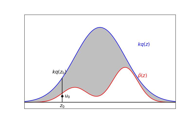
<h1 id="4-conclusion-and-whats-next">4. Conclusion and What’s Next</h1>

<p>In this post, we’ve introduced a more versatile sampling method than rejection sampling. We implemented rejection sampling in Python and used the example to better understand the implications of importance sampling.</p>

<p>In the next post, we’ll explore a more universal approach using the Metropolis Hastings Algorithm with Markov Chains</p>]]></content><author><name>Hans Nusspickel</name></author><summary type="html"><![CDATA[1. Introduction to Importance Sampling]]></summary></entry><entry><title type="html">Rejection Sampling</title><link href="https://hanusspi.github.io/2024/08/18/RejectionSampling.html" rel="alternate" type="text/html" title="Rejection Sampling" /><published>2024-08-18T00:00:00+00:00</published><updated>2024-08-18T00:00:00+00:00</updated><id>https://hanusspi.github.io/2024/08/18/RejectionSampling</id><content type="html" xml:base="https://hanusspi.github.io/2024/08/18/RejectionSampling.html"><![CDATA[<h1 id="1-introduction-to-rejection-sampling">1. Introduction to Rejection Sampling</h1>

<p>When dealing with complex probability distributions \(p(z)\), direct sampling can be difficult or even impossible. This is where we can use Rejection Sampling, which allows us to sample from a complex distribution with the aid of a proposal distribution, that we can evaluate.</p>

<p>Rejection sampling is especially useful in Bayesian inference when dealing with non-standard distributions that don’t have a straightforward method for drawing samples. In this post, we’ll explore the concept of rejection sampling.</p>

<h1 id="2-why-rejection-sampling">2. Why Rejection Sampling?</h1>

<p>Rejection sampling is used when:</p>

<ul>
  <li>
    <p>Direct Sampling is Difficult: When we can’t easily sample from the target distribution, rejection sampling provides an alternative method.</p>
  </li>
  <li>
    <p>Target Distribution is Known Up to a Constant: To perform rejection sampling, we need to be able to evaluate the target distribution to some normalization factor \(Z_p\)
\(p(z) = \frac{1}{Z_p}\tilde{p}(z)\)
Preferably with very little effort.</p>
  </li>
</ul>

<h1 id="3-how-rejection-sampling-works">3. How Rejection Sampling Works</h1>

<p>The idea of rejection sampling is to sample from a proposal distribution and then “reject” or “accept” samples based on how likely they are under the target distribution.</p>

<p><img src="/img/posts/2024-08-17-RejectionSampling/rejectionIdea.jpg" alt="Imagetext" /></p>

<p>Let’s break it down into simple steps:</p>

<ol>
  <li>
    <p>Choose a Proposal Distribution: Select a proposal distribution \(q(z)\) that is easy to sample from and that roughly covers the shape of the target distribution \(\tilde{p}(z)\). The proposal distribution should be scaled by a constant \(k\), such that \(\forall z: kq(x) \geq \tilde{p}(z)\).</p>
  </li>
  <li>
    <p>Generate a Sample: Draw a sample \(z\) from the proposal distribution \(q(z)\).</p>
  </li>
  <li>
    <p>Generate a Uniform Random Variable: Draw a uniform random variable \(u\) from \(\operatorname{Uniform}(0,1)\).</p>
  </li>
  <li>
    <p>Acceptance Criterion: Accept the sample \(z\) if \(u\leq\frac{\tilde{p}(z)}{kq(z)}\)​. If not, reject the sample and go back to step 2.</p>
  </li>
  <li>
    <p>Repeat: Continue the process until you have enough accepted samples.</p>
  </li>
</ol>

<p>The accepted samples will be approximately distributed according to the target distribution \(p(x)\).</p>

<h1 id="4-example-rejection-sampling-from-a-gaussian-mixture-model">4. Example: Rejection Sampling from a Gaussian Mixture Model</h1>

<p>Let’s now consider an example where we want to sample from a Gaussian Mixture Model (GMM), which is a combination of multiple Gaussian distributions as a demonstration.</p>

<p>We’ll use a simple GMM composed of two Gaussian distributions.</p>

<p>The target distribution \(p(x)\) is a mixture of two Gaussian distributions:
\(p(x)=0.3\cdot \mathcal{N}(x;−2,0.5^2)+0.7\cdot \mathcal{N}(x;2,1^2)\)</p>

<p>The normalization factor \(Z_p\) in this case is 1, since we can evaluate this function precisly.</p>

<p>We will use a simple normal distribution as the proposal distribution \(q(x)\).</p>

<ol>
  <li>Python Code Example: Rejection Sampling</li>
</ol>

<figure class="highlight"><pre><code class="language-python" data-lang="python"><table class="rouge-table"><tbody><tr><td class="gutter gl"><pre class="lineno">1
2
3
4
5
6
7
8
9
10
11
12
13
14
15
16
17
18
19
20
21
22
23
24
25
26
27
28
29
30
31
32
33
34
35
36
37
38
39
40
41
42
</pre></td><td class="code"><pre><span class="kn">import</span> <span class="nn">numpy</span> <span class="k">as</span> <span class="n">np</span>
<span class="kn">import</span> <span class="nn">matplotlib.pyplot</span> <span class="k">as</span> <span class="n">plt</span>
<span class="kn">from</span> <span class="nn">scipy.stats</span> <span class="kn">import</span> <span class="n">norm</span>

<span class="c1"># Define the target distribution (Gaussian Mixture Model)
</span><span class="k">def</span> <span class="nf">target_distribution</span><span class="p">(</span><span class="n">x</span><span class="p">):</span>
    <span class="k">return</span> <span class="mf">0.3</span> <span class="o">*</span> <span class="n">norm</span><span class="p">.</span><span class="n">pdf</span><span class="p">(</span><span class="n">x</span><span class="p">,</span> <span class="o">-</span><span class="mi">2</span><span class="p">,</span> <span class="mf">0.5</span><span class="p">)</span> <span class="o">+</span> <span class="mf">0.7</span> <span class="o">*</span> <span class="n">norm</span><span class="p">.</span><span class="n">pdf</span><span class="p">(</span><span class="n">x</span><span class="p">,</span> <span class="mi">2</span><span class="p">,</span> <span class="mf">1.0</span><span class="p">)</span>

<span class="c1"># Define the proposal distribution (Normal distribution)
</span><span class="n">proposal_distribution</span> <span class="o">=</span> <span class="n">norm</span><span class="p">(</span><span class="mi">0</span><span class="p">,</span> <span class="mi">3</span><span class="p">)</span>  <span class="c1"># Mean 0, std 3
</span>
<span class="c1"># Define the constant M such that M * proposal_distribution &gt;= target_distribution
</span><span class="n">M</span> <span class="o">=</span> <span class="mf">1.5</span>  <span class="c1"># Chosen to ensure the proposal upper-bounds the target
</span>
<span class="c1"># Number of samples
</span><span class="n">n_samples</span> <span class="o">=</span> <span class="mi">10000</span>

<span class="c1"># Rejection Sampling
</span><span class="n">samples</span> <span class="o">=</span> <span class="p">[]</span>
<span class="k">while</span> <span class="nb">len</span><span class="p">(</span><span class="n">samples</span><span class="p">)</span> <span class="o">&lt;</span> <span class="n">n_samples</span><span class="p">:</span>
    <span class="n">x</span> <span class="o">=</span> <span class="n">proposal_distribution</span><span class="p">.</span><span class="n">rvs</span><span class="p">()</span>  <span class="c1"># Sample from proposal distribution
</span>    <span class="n">u</span> <span class="o">=</span> <span class="n">np</span><span class="p">.</span><span class="n">random</span><span class="p">.</span><span class="n">uniform</span><span class="p">(</span><span class="mi">0</span><span class="p">,</span> <span class="mi">1</span><span class="p">)</span>  <span class="c1"># Uniform random variable
</span>
    <span class="c1"># Accept or reject the sample
</span>    <span class="k">if</span> <span class="n">u</span> <span class="o">&lt;=</span> <span class="n">target_distribution</span><span class="p">(</span><span class="n">x</span><span class="p">)</span> <span class="o">/</span> <span class="p">(</span><span class="n">M</span> <span class="o">*</span> <span class="n">proposal_distribution</span><span class="p">.</span><span class="n">pdf</span><span class="p">(</span><span class="n">x</span><span class="p">)):</span>
        <span class="n">samples</span><span class="p">.</span><span class="n">append</span><span class="p">(</span><span class="n">x</span><span class="p">)</span>

<span class="c1"># Convert to numpy array for easier handling
</span><span class="n">samples</span> <span class="o">=</span> <span class="n">np</span><span class="p">.</span><span class="n">array</span><span class="p">(</span><span class="n">samples</span><span class="p">)</span>

<span class="c1"># Plot the histogram of the samples
</span><span class="n">plt</span><span class="p">.</span><span class="n">figure</span><span class="p">(</span><span class="n">figsize</span><span class="o">=</span><span class="p">(</span><span class="mi">10</span><span class="p">,</span> <span class="mi">6</span><span class="p">))</span>
<span class="n">plt</span><span class="p">.</span><span class="n">hist</span><span class="p">(</span><span class="n">samples</span><span class="p">,</span> <span class="n">bins</span><span class="o">=</span><span class="mi">50</span><span class="p">,</span> <span class="n">density</span><span class="o">=</span><span class="bp">True</span><span class="p">,</span> <span class="n">alpha</span><span class="o">=</span><span class="mf">0.6</span><span class="p">,</span> <span class="n">color</span><span class="o">=</span><span class="s">'b'</span><span class="p">,</span> <span class="n">label</span><span class="o">=</span><span class="s">"Sampled Data"</span><span class="p">)</span>

<span class="c1"># Overlay the target distribution
</span><span class="n">x</span> <span class="o">=</span> <span class="n">np</span><span class="p">.</span><span class="n">linspace</span><span class="p">(</span><span class="o">-</span><span class="mi">6</span><span class="p">,</span> <span class="mi">6</span><span class="p">,</span> <span class="mi">1000</span><span class="p">)</span>
<span class="n">plt</span><span class="p">.</span><span class="n">plot</span><span class="p">(</span><span class="n">x</span><span class="p">,</span> <span class="n">target_distribution</span><span class="p">(</span><span class="n">x</span><span class="p">),</span> <span class="s">'r'</span><span class="p">,</span> <span class="n">linewidth</span><span class="o">=</span><span class="mi">2</span><span class="p">,</span> <span class="n">label</span><span class="o">=</span><span class="s">"Target Distribution"</span><span class="p">)</span>
<span class="n">plt</span><span class="p">.</span><span class="n">title</span><span class="p">(</span><span class="s">"Rejection Sampling from a Gaussian Mixture Model"</span><span class="p">)</span>
<span class="n">plt</span><span class="p">.</span><span class="n">xlabel</span><span class="p">(</span><span class="s">"Value"</span><span class="p">)</span>
<span class="n">plt</span><span class="p">.</span><span class="n">ylabel</span><span class="p">(</span><span class="s">"Density"</span><span class="p">)</span>
<span class="n">plt</span><span class="p">.</span><span class="n">legend</span><span class="p">()</span>
<span class="n">plt</span><span class="p">.</span><span class="n">show</span><span class="p">()</span>
</pre></td></tr></tbody></table></code></pre></figure>

<p><img src="/img/posts/2024-08-17-RejectionSampling/rejectionSampling.jpg" alt="Imagetext" /></p>

<h1 id="5-limitations-of-rejection-sampling">5. Limitations of Rejection Sampling</h1>

<p>Now that we gained a rough understanding of how rejection sampling works, we can see that it can be very usefull, but there are also some obvious limitations:</p>

<ul>
  <li>Efficiency: Rejection sampling can be inefficient if the proposal distribution doesn’t closely match the target distribution. The more samples we reject, the longer it takes to generate enough accepted samples.</li>
  <li>Parameters: Rejection Sampling cannot be simply used. For every usecase we need to find a good matching proposal distribution, which in itself can be very challenging or risk loosing alot of efficiency.</li>
  <li>Dimensionality: In high-dimensional spaces, finding a suitable proposal distribution that covers the target distribution well can be even more challenging, leading to high rejection rates.</li>
</ul>

<h1 id="conclusion-and-whats-next">Conclusion and What’s Next</h1>

<p>In this post, we’ve introduced the concept of rejection sampling, a versatile technique for sampling from complex distributions. We implemented rejection sampling in Python and visualized how the method works in practice. Rejection sampling is a powerful tool but comes with trade-offs in terms of efficiency and complexity.</p>

<p>In the next post, we’ll explore Importance Sampling, a related method that improves efficiency by weighting samples from the proposal distribution instead of rejecting them.</p>]]></content><author><name>Hans Nusspickel</name></author><summary type="html"><![CDATA[1. Introduction to Rejection Sampling]]></summary></entry><entry><title type="html">Sampling from a Distribution</title><link href="https://hanusspi.github.io/2024/08/17/SamplingFromADistribution.html" rel="alternate" type="text/html" title="Sampling from a Distribution" /><published>2024-08-17T00:00:00+00:00</published><updated>2024-08-17T00:00:00+00:00</updated><id>https://hanusspi.github.io/2024/08/17/SamplingFromADistribution</id><content type="html" xml:base="https://hanusspi.github.io/2024/08/17/SamplingFromADistribution.html"><![CDATA[<h1 id="1-introduction-to-sampling">1. Introduction to Sampling</h1>

<p>Sampling is a foundational concept in statistics and machine learning, and it plays a crucial role in Bayesian inference, particularly in approximate methods. Simply put, sampling involves drawing random values from a probability distribution. These samples can be used to estimate properties of the distribution, such as its mean, variance, or other moments.</p>

<p>In this post, we’ll explore the basics of sampling, its significance in Bayesian inference, and how to perform sampling from a specific distribution using the Inverse Transform Sampling technique.</p>
<h1 id="2-why-sampling-is-important-in-inference">2. Why Sampling is Important in Inference</h1>

<p>Sampling is essential in approximate inference methods, especially when dealing with complex models where exact analytical solutions are not feasible. It allows us to estimate expectations, probabilities, and other quantities by drawing samples from the desired distribution.</p>

<p>This is crucial in many applications, including:</p>

<ul>
  <li>Monte Carlo Methods: Approximating expectations using random samples.</li>
  <li>Bayesian Inference: Sampling from the posterior distribution when it cannot be computed analytically.</li>
  <li>Optimization: Exploring complex probability landscapes using sampling techniques.</li>
</ul>

<p>In this post, we’ll focus on a practical example of sampling from an exponential distribution using Python.</p>
<h1 id="3-the-exponential-distribution">3. The Exponential Distribution</h1>

<p>The exponential distribution is a common distribution used to model the time between independent events that happen at a constant average rate. It is characterized by the rate parameter \(λ\).</p>

<p>The probability density function (PDF) of the exponential distribution is given by:
\(f(x;λ)=λe−λxforx≥0\)</p>

<p>where \(λ\) is the rate parameter.</p>

<p>The cumulative distribution function (CDF) is the integral of the PDF:
\(F(x;λ)=1−e−λx\)</p>

<p>Using the inverse of this CDF, we can sample from the exponential distribution using a uniform random variable.</p>

<h1 id="4-inverse-transform-sampling">4. Inverse Transform Sampling</h1>

<p>Inverse Transform Sampling is a method to generate random samples from a given distribution by inverting its CDF. The steps are:</p>

<p>Generate a uniform random variable \(u∼Uniform(0,1)\).
Compute the inverse of the CDF at uu to obtain the corresponding sample \(x\).</p>

<p>For the exponential distribution, the CDF is:
\(F(x;λ)=1−e−λx\)</p>

<p>To invert this, solve for xx:
\(u=1−e−λx\)
\(e−λx=1−u\)
\(x=−1λln⁡(1−u)\)</p>

<p>Thus, to generate a sample from the exponential distribution, we can use the formula:
\(x=−1λln⁡(1−u)\)</p>

<h1 id="5-python-code-example-sampling-from-an-exponential-distribution">5. Python Code Example: Sampling from an Exponential Distribution</h1>

<p>Here’s how you can implement inverse transform sampling for the exponential distribution in Python:</p>

<figure class="highlight"><pre><code class="language-python" data-lang="python"><table class="rouge-table"><tbody><tr><td class="gutter gl"><pre class="lineno">1
2
3
4
5
6
7
8
9
10
11
12
13
14
15
16
17
18
19
20
21
22
23
24
25
26
27
</pre></td><td class="code"><pre><span class="kn">import</span> <span class="nn">numpy</span> <span class="k">as</span> <span class="n">np</span>
<span class="kn">import</span> <span class="nn">matplotlib.pyplot</span> <span class="k">as</span> <span class="n">plt</span>

<span class="c1"># Define the rate parameter lambda
</span><span class="n">lambda_param</span> <span class="o">=</span> <span class="mf">1.0</span>

<span class="c1"># Number of samples
</span><span class="n">n_samples</span> <span class="o">=</span> <span class="mi">1000</span>

<span class="c1"># Generate uniform random variables
</span><span class="n">u</span> <span class="o">=</span> <span class="n">np</span><span class="p">.</span><span class="n">random</span><span class="p">.</span><span class="n">uniform</span><span class="p">(</span><span class="mi">0</span><span class="p">,</span> <span class="mi">1</span><span class="p">,</span> <span class="n">n_samples</span><span class="p">)</span>

<span class="c1"># Inverse transform sampling to generate samples from the exponential distribution
</span><span class="n">samples</span> <span class="o">=</span> <span class="o">-</span><span class="n">np</span><span class="p">.</span><span class="n">log</span><span class="p">(</span><span class="mi">1</span> <span class="o">-</span> <span class="n">u</span><span class="p">)</span> <span class="o">/</span> <span class="n">lambda_param</span>

<span class="c1"># Plot the histogram of the samples
</span><span class="n">plt</span><span class="p">.</span><span class="n">figure</span><span class="p">(</span><span class="n">figsize</span><span class="o">=</span><span class="p">(</span><span class="mi">10</span><span class="p">,</span> <span class="mi">6</span><span class="p">))</span>
<span class="n">plt</span><span class="p">.</span><span class="n">hist</span><span class="p">(</span><span class="n">samples</span><span class="p">,</span> <span class="n">bins</span><span class="o">=</span><span class="mi">30</span><span class="p">,</span> <span class="n">density</span><span class="o">=</span><span class="bp">True</span><span class="p">,</span> <span class="n">alpha</span><span class="o">=</span><span class="mf">0.6</span><span class="p">,</span> <span class="n">color</span><span class="o">=</span><span class="s">'b'</span><span class="p">)</span>
<span class="n">plt</span><span class="p">.</span><span class="n">title</span><span class="p">(</span><span class="s">"Sampling from an Exponential Distribution using Inverse Transform Sampling"</span><span class="p">)</span>
<span class="n">plt</span><span class="p">.</span><span class="n">xlabel</span><span class="p">(</span><span class="s">"Value"</span><span class="p">)</span>
<span class="n">plt</span><span class="p">.</span><span class="n">ylabel</span><span class="p">(</span><span class="s">"Density"</span><span class="p">)</span>

<span class="c1"># Overlay the true exponential distribution
</span><span class="n">x</span> <span class="o">=</span> <span class="n">np</span><span class="p">.</span><span class="n">linspace</span><span class="p">(</span><span class="mi">0</span><span class="p">,</span> <span class="mi">8</span><span class="p">,</span> <span class="mi">1000</span><span class="p">)</span>
<span class="n">plt</span><span class="p">.</span><span class="n">plot</span><span class="p">(</span><span class="n">x</span><span class="p">,</span> <span class="n">lambda_param</span> <span class="o">*</span> <span class="n">np</span><span class="p">.</span><span class="n">exp</span><span class="p">(</span><span class="o">-</span><span class="n">lambda_param</span> <span class="o">*</span> <span class="n">x</span><span class="p">),</span> <span class="s">'r'</span><span class="p">,</span> <span class="n">linewidth</span><span class="o">=</span><span class="mi">2</span><span class="p">,</span> <span class="n">label</span><span class="o">=</span><span class="s">'True PDF'</span><span class="p">)</span>
<span class="n">plt</span><span class="p">.</span><span class="n">legend</span><span class="p">()</span>
<span class="n">plt</span><span class="p">.</span><span class="n">show</span><span class="p">()</span>
</pre></td></tr></tbody></table></code></pre></figure>

<p><img src="img/posts/2024-08-16-SamplingFromADistribution/samplingFromDistr.jpg" alt="Imagetext" /></p>

<h1 id="6-applications-of-sampling">6. Applications of Sampling</h1>

<p>Sampling isn’t just a theoretical exercise; it has practical applications in various domains:</p>

<ul>
  <li>Monte Carlo Methods: Sampling forms the basis of Monte Carlo methods, which are used to estimate integrals, simulate systems, and perform Bayesian inference.</li>
  <li>Bootstrap Methods: In statistics, sampling is used in bootstrap methods to estimate the sampling distribution of a statistic by resampling from the data.</li>
  <li>MCMC Algorithms: Markov Chain Monte Carlo methods rely heavily on sampling to explore complex posterior distributions.</li>
</ul>

<p>These applications show how sampling is a versatile tool in both statistics and machine learning.</p>

<h1 id="conclusion-and-whats-next">Conclusion and What’s Next</h1>

<p>In this post, we’ve introduced sampling from the exponential distribution using the Inverse Transform Sampling technique. Sampling is a crucial technique in Bayesian inference, especially when exact solutions are not feasible.</p>

<p>In the next post, we’ll dive into Rejection Sampling, a powerful method for sampling from complex distributions when direct sampling is difficult.</p>]]></content><author><name>Hans Nusspickel</name></author><summary type="html"><![CDATA[1. Introduction to Sampling]]></summary></entry><entry><title type="html">Introduction to Approximate Inference</title><link href="https://hanusspi.github.io/2024/08/16/Approximate-Interence.html" rel="alternate" type="text/html" title="Introduction to Approximate Inference" /><published>2024-08-16T00:00:00+00:00</published><updated>2024-08-16T00:00:00+00:00</updated><id>https://hanusspi.github.io/2024/08/16/Approximate-Interence</id><content type="html" xml:base="https://hanusspi.github.io/2024/08/16/Approximate-Interence.html"><![CDATA[<h1 id="1-what-is-bayesian-inference">1. What is Bayesian Inference?</h1>

<p>Bayesian inference is a powerful statistical technique that allows us to update our beliefs about the world as we gather more evidence. Unlike classical (frequentist) approaches, which often focus on fixed parameters and p-values, Bayesian inference provides a probabilistic framework where uncertainty is quantified and incorporated into the analysis.</p>

<p>At its core, Bayesian inference is built upon Bayes’ Theorem:</p>

\[P(H|D) = \frac{P(D|H)\cdot P(H)}{P(D)}\]

<ul>
  <li>\(P(H \vert D)\): The posterior probability, which represents our updated belief in the hypothesis H after observing data \(D\).</li>
  <li>\(P(D \vert H)\): The likelihood, the probability of the data given that the hypothesis \(H\) is true.</li>
  <li>\(P(H)\): The prior probability, which represents our initial belief in the hypothesis before seeing the data.</li>
  <li>\(P(D)\): The evidence or marginal likelihood, which is the total probability of observing the data under all possible hypotheses.</li>
</ul>

<p>Bayesian inference is particularly useful when dealing with uncertainty, incorporating prior knowledge, and updating beliefs as new information becomes available.</p>

<h1 id="2-exact-vs-approximate-inference">2. Exact vs. Approximate Inference</h1>

<p>While Bayesian inference provides a robust framework, it can be computationally challenging. In simple cases, we can calculate the posterior distribution exactly, which is known as exact Bayesian inference. However, in more complex models, calculating the exact posterior distribution becomes intractable due to high-dimensional integrals or complex likelihood functions.</p>

<p>This is where approximate inference comes into play. Approximate methods aim to estimate the posterior distribution without solving it exactly. These methods allow us to perform Bayesian inference in situations where exact methods would be computationally impossible.</p>

<p>Here’s a brief comparison:</p>

<ul>
  <li>Exact Inference:
    <ul>
      <li>Pros: Provides precise posterior distributions.</li>
      <li>Cons: Computationally expensive or impossible for complex models.</li>
    </ul>
  </li>
  <li>Approximate Inference:
    <ul>
      <li>Pros: Scalable to complex models and large datasets.</li>
      <li>Cons: Introduces approximations, which may lead to less precise results.</li>
    </ul>
  </li>
</ul>

<p>This blog series will dive into several approximate methods, but before we do, let’s walk through a simple example of exact Bayesian inference.</p>

<h1 id="3-example-of-exact-bayesian-inference">3. Example of Exact Bayesian Inference</h1>
<p>Let’s consider a classic problem in Bayesian statistics: estimating the probability of a coin being biased.</p>

<p>Imagine you have a coin, and you’re not sure whether it’s fair (i.e., whether it lands heads or tails with equal probability). You decide to model this uncertainty using Bayesian inference.</p>

<ul>
  <li>
    <p>Prior Belief: You believe that the coin is probably fair, but you’re open to the possibility that it might be biased. This belief can be represented by a Beta distribution, a common choice for modeling probabilities.</p>
  </li>
  <li>
    <p>Data: You flip the coin 10 times and observe 7 heads.</p>
  </li>
  <li>
    <p>Likelihood: The likelihood function here is binomial since we’re counting the number of successes (heads) in a fixed number of trials (10 flips).</p>
  </li>
  <li>
    <p>Posterior Distribution: Using Bayes’ Theorem, we update our belief about the fairness of the coin.</p>
  </li>
</ul>

<p>Here’s the Python code that performs exact Bayesian inference for this problem:</p>

<figure class="highlight"><pre><code class="language-python" data-lang="python"><table class="rouge-table"><tbody><tr><td class="gutter gl"><pre class="lineno">1
2
3
4
5
6
7
8
9
10
11
12
13
14
15
16
17
18
</pre></td><td class="code"><pre><span class="kn">import</span> <span class="nn">numpy</span> <span class="k">as</span> <span class="n">np</span>
<span class="kn">import</span> <span class="nn">matplotlib.pyplot</span> <span class="k">as</span> <span class="n">plt</span>
<span class="kn">from</span> <span class="nn">scipy.stats</span> <span class="kn">import</span> <span class="n">beta</span>

<span class="c1"># Define prior: Beta(2, 2) (initial belief that the coin is fair)
</span><span class="n">a_prior</span> <span class="o">=</span> <span class="mi">2</span>
<span class="n">b_prior</span> <span class="o">=</span> <span class="mi">2</span>

<span class="c1"># Data: 7 heads out of 10 flips
</span><span class="n">heads</span> <span class="o">=</span> <span class="mi">7</span>
<span class="n">tails</span> <span class="o">=</span> <span class="mi">3</span>

<span class="c1"># Posterior distribution parameters: Beta(a + heads, b + tails)
</span><span class="n">a_post</span> <span class="o">=</span> <span class="n">a_prior</span> <span class="o">+</span> <span class="n">heads</span>
<span class="n">b_post</span> <span class="o">=</span> <span class="n">b_prior</span> <span class="o">+</span> <span class="n">tails</span>

<span class="c1"># Generate x values for plotting
</span><span class="n">x</span> <span class="o">=</span> <span class="n">np</span><span class="p">.</span><span class="n">linspace</span><span class="p">(</span><span class="mi">0</span><span class="p">,</span> <span class="mi">1</span><span class="p">,</span> <span class="mi">100</span><span class="p">)</span>
</pre></td></tr></tbody></table></code></pre></figure>

<p><img src="\img\posts\2024-08-16-Approximate-Inference\exactBayesianInference.png" alt="Imagetext" /></p>

<h1 id="4-motivation-for-approximate-inference">4. Motivation for Approximate Inference</h1>

<p>While the above example was simple, imagine trying to apply exact Bayesian inference to a model with thousands of parameters or complex data structures. In these cases, computing the exact posterior distribution might require solving high-dimensional integrals, which is often infeasible.</p>

<p>This is where approximate inference methods come into play. These methods provide ways to estimate the posterior distribution without needing to compute it exactly. In the upcoming posts, we’ll explore several key techniques for approximate inference, including:</p>

<ul>
  <li>Sampling Methods: Techniques like rejection sampling, importance sampling, and Markov Chain Monte Carlo (MCMC).</li>
  <li>Variational Methods: Approximating the posterior with simpler distributions.</li>
  <li>Latent Variable Models: Inference in models with hidden variables.</li>
</ul>

<p>These methods are not just theoretical tools; they are essential for modern machine learning and data science applications, from probabilistic models to deep learning.</p>

<h1 id="conclusion">Conclusion:</h1>

<p>Bayesian inference is a foundational concept in statistics and machine learning, allowing us to update our beliefs as new data arrives. However, the complexity of real-world problems often necessitates approximate methods. In this blog series, we’ll embark on a journey to understand these methods, starting with basic sampling techniques and progressing to more advanced topics like MCMC and variational inference.</p>

<p>Stay tuned for the next post, where we’ll dive into the basics of sampling from a distribution!</p>]]></content><author><name>Hans Nusspickel</name></author><summary type="html"><![CDATA[1. What is Bayesian Inference?]]></summary></entry></feed>