1. Introduction
In the last post we created our first pressure solver and got some pretty good results. Real fluids though do not really look like a bunch of spheres, but have a closed fluid surface. To resolve this issue, we define a function that can tell us how far a point in space is from the fluid surface. To do this we will define a signed distance function, that works with the lagrangian fluid simulation. Furthermore we need a strategy to create points, for which we can sample the distance to the surface and turn those points into a grid. And this is what we will start with.
2. Marching Cubes
To start off with marching cubes algorighm [LC87] we overlay the simulation domain with a voxel grid. The length of a voxel we will denote with \(l\). Next we sample some function, in most cases a signed distance field (sdf) \(\Phi\) at each corner point \(x_i\) of each voxel.
The first major issue of this algorithm is indexing. We have a 3d voxel grid, but need to store everything in a 1d array. Therefore we determine unique integer coordinates (i,j,k) (which are easy to translate into world space) with (0,0,0) at the origin of the grid. Given the size of our simulation domain, which we can represent as an Axis Aligned Bounding Box (AABB) we can determine how many voxel cells the grid has in each dimension, denoted by \(n_x, n_y, n_z\). Next we need to map each integer coordinate to a vertex (corner of a voxel) with
\(V = in_y n_z + j n_z + k\).
In the same fashion a cell can be identified with
\(C = in_y n_z + j n_z + k\).
Even though we have one less cell in each direction than vertices. But for simplicity we keep it like that.
And lastly we need a function to define edges
\[E = 3 V + dir,\]where dir is 0,1,2 for x,y,z.
For the full implementation we will have to handle some literal edge cases, because vertices on the outer side of the grid do not have edges in all directions.
The nice thing about those functions is, that they are bijective, therefore from a vertex id we can backtrack to its integer and finally world coordinates. Given the world coordinate x we can sample \(\phi(x)\) and get for the vertex i \(\Phi_i = \Phi(x_i)\).
With this information we know if a vertex is inside or outside of the surface. This already gives us some basic information, but not a mesh yet.
Therefore next we will iterate over all edges and check if they intersect the surface, i.e. if the sign between the vertices making up the edge changes. If we have a sign change, we calculate an edge weight by linear interpolation giving us the intersection point. This gives us a solid guess of where the actual surface could be. It is important that we store these points in relation to the edge they belong to. Since our surface is going to have a lot fewer points than we have voxels, it is sensible to store them in a map.
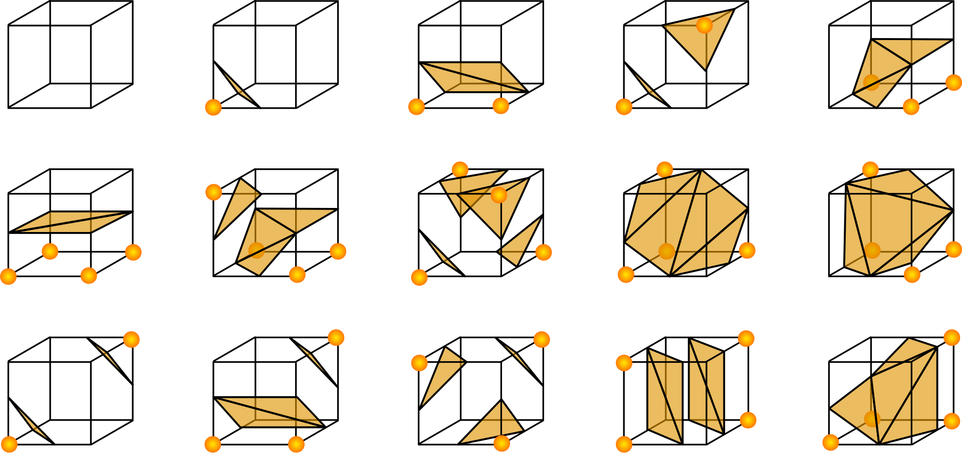
In the last step we need to append the vertex data with geometric connectivity. For this a marching cubes table exists, that we can use. As visible in the image above, the marching cube table tells us, based on which edges experiencing a sign change, which vertices to connect. And for this to work properly, all the previous hassle with indexing was required.
Lastly, to get a smooth mesh, we do not just need to have vertices and connectivity, but also vertex normals. These we can either calculate in the beginning for the voxel corners and interpolate later on or calculate in a second sweep for the exact vertex positions.
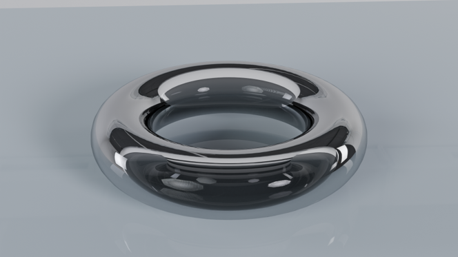
Applying this for an object with a known signed distance function, like a torus yields this result:
3. Fluid Surface Reconstruction
To make marching cubes work we therefore need a \(\Phi\) that we can sample. While for primitive shapes, like a torus, sphere or square these are analytically defined, for our fluid they are not. Therefore we need a function that is close to 1, if it is inside the fluid and 0 or even negative if it is outside of the fluid. Applying some fundamentals of the SPH idea and using the method how we determine the value of quantites in SPH (as discusses in the last posts) gives us [BJ25]
\[\Phi(\mathbf{x})=-c+\sum_{j\in\mathcal{N}(\mathbf{x})}\frac{1}{\rho_j}W(\mathbf{x}-\mathbf{x}_j,h),\]where \(\rho_j\) is now the normalized density estimation
\[\rho_i=\sum_{j\in\mathcal{N}(\mathbf{x}_i)}W(\mathbf{x}_i-\mathbf{x}_j,h).\]We are required to add a slightly negative c to force a sign change, since the second part of the function will never get smaller than 0. By choosing the c we can determine how tight or loose we want the surface to be. A good starting value is 0.55.
Since this formulation seemingly requires a neighborhood search, it seems to be pretty expensive. Since unlike the particles, our vertices are grid aligned and indexable though, we can turn things around and iterate over the particles, determine an AABB around each particle, check which vertices are in the interior of the AABB and then write the values to the vertices. The only disadvantage of this approach is that it is very hard to parallelize.
In the very beginning we defined the cell size as a parameter. We want to set the cell size so that a sole particle can create a single mesh, to prevent particles suddenly popping up and vanishing later on. Therefore a good cell size is 1.0 times the particle radius.
4. Results
Applying marching cubes and the newly defined sdf gives us this lovely result for our previously generated simulation
Depending on the rendering settings in Blender the look of the fluid can be varied even further.
5. Summary
In this post we started out by defining a voxel grid with many indices turning it into the marching cube algorithm [LC87]. Finally we managed to apply it to a particle based fluid simulation turning it into a real fluid. The code can be found under https://github.com/hanusspi/BasicPressureSolverLab, where the mesh gets generated as a vtk and can be imported into blender using the same workflow as for the particles in the previous blog post.
References
[LC87] W.E. Lorensen and H.E. Cline. Marching cubes: A high resolution 3d surface construction algorithm. ACM Computer Graphics, 21(4):163–169, 1987. [BJ25] Prof. Dr. Jan Bender, M.Sc. Timna B¨ottcher, M.Sc. Jos´e Fern´andez, M.Sc. Lukas Westhofen: Fluid Simulation in Computer Graphics