1. Bayes to MCMC: Recap

So far we have discussed bayesian analysis of data. So we took data, a hypothesis and prior knowledge to gain an insight on the posterior. For this we considered rejection sampling and importance sampling, which were both absed on independent samples from q(z). However, for many problems of practical interests, is is difficult or even impossible to find a fitting q(z) with the required accuracy.

For that reason it would be better to simply abondon independent sampling and simply rely on a stochastic process to generate dependent samples from the target distribution. For this we use a Markov Chain and a Monte Carlo estimate. This might sound a bit abstrct for now, but in a bit we will figure out how this works in detail.

The core topic is now called MCMC (Markov Chain Monte Carlo) and allows us to sample from a large class of distributions. For this a new sample is generated within a probability distribution of the previous sample in the chain. MCMC is popular, as it scales better with higher dimensions.

For a Markov Chain we have a set of states and a state transition relation. Futher more the state transitions can have different probabilites. Now we keep a record tof the current state \(z^{(\tau)}\) and the proposal distribution depends on the current state: \(q(z|z^{(\tau)})\). The sequence of samples from the chain we will denote with \(z^{(1)}, z^{(2)},...\) and again we assume, that we can evaluate \(p(z) = \frac{1}{Z_p}\tilde{p}(z)\). Now at each time step, we generate a candidate sample from the proposal distribution and accept the sample according to a criterion.

2. Metropolis-Hastings Algorighm

The idea of MCMC is that the chainis a sequence of states created through iterative estimations of new states. A state is a set of parameters of an analytic model over which MCMC is iterating in order to maximize the posterior. For a markov chain, the markov property has to hold: \(P[S|S'] = P[S|S',S'']\) . So the probability of state \(S\) only depends on the previous state \(S'\) and not on any other earlier visited states. In the Bayesian context, the accpetance of a new state often involves comparing the likelihood of the current state, with respect to a uniformly sampled acceptance threshold. This might sound a bit confusing in the beginning but will become clearer in the code.

For now lets assume, that the proposal distribution is symmetric, therefore \(q(z_A|z_B) = q(z_B|z_A)\) holds. Now we need to determine the probability with which we accept a new candidate sample \(z^*\) :

Now we can again sample \(u\) from a uniform distribution and accept the sample, if \(A(z^*, z^{(\tau)}) > u\) . What we can already note is, that the new candiate sample will always be accepted if \(\tilde{p}(z^*) \geq \tilde{p}^{(\tau)}\) . So if the new sample has a higher probability than the previous one, we will accpet it. But every now and then the algorithm also accpets samples with lower probability. For the next step this means, that if the new sample is accepted, that \(z^{(\tau+1)} = z^*\) and if the new sample is not accepted, \(z^{(\tau+1)} = z^{(\tau)}\) . If we compare this to rejection sampling, we discarded rejected samples. Now we still discard samples, but copy accepted samples in return. So there can be multiple copies of a sample. This simpler case is the original Metropolis Algorithm and has the property, that if \(q(z_A|z_B)>0\) for all \(z\) , the distribution of \(z^{\tau}\) tends to \(p(z)\) as \(\tau \rightarrow \inf\) .

To compensate for non symmetric proposal distributions, we can append to our acceptance probability and define it with:

where k labels the members of the set of possible transitions considered. The evaluation of the acceptance criterion does not require the normalizing constant \(Z_p\) . And now we can also see, that if \(q_k\) is symmetrical, Metropolis Hastings becomes the Metropolis Algorithm.

3. Implementation in Python

For our implementation example lets stay with a 1D mixture of gausisians as given for the previous sampling methods. Furthermore we will use a simple gaussian as proposal distribution. Lets start by defining the distributions:

1
2
3
4
5
6
7
8
9
10
11
12
def gaussian(x, mu, sigma):
    factor = 1 / (sigma * np.sqrt(2 * np.pi))
    return factor * np.exp(-0.5 * ((x - mu) / sigma) ** 2)

def target(x):
    return 0.3 * norm.pdf(x, 0, 2) + 0.7 * norm.pdf(x, 10, 2)

def proposal(mu, sigma):
    return mu + sigma * np.random.randn()

def proposal_conditional(x, y, sigma_prop):
    return gaussian(x=x, mu=y, sigma=sigma_prop)

This style of formulating the distributions seems a bit weird, but makes sense, since i wanted to play around a bit with the functools.partial() function, which turns a parametrized function into a predefined function for fixed inputs. Next take a look at the Metropolis Hastings Algorithm:

1
2
3
4
5
6
7
8
9
10
11
12
13
14
15
16
17
18
19
20
21
22
23
24
25
26
def MH(target, proposal, proposal_conditional, n_iterations):
    samples = []
    n_accepted = 0

    # initial state
    x = np.random.rand()
    proposal_old = target(x)

    for i in range(n_iterations):
        xprime = proposal(x)    
        proposal_new = target(xprime) # P(x')
        alpha = proposal_new / (proposal_old + np.finfo(float).eps) # P(x') / P(x)
        alpha *= proposal_conditional(x, xprime) / proposal_conditional(xprime, x) # q(x|x’), q(x'|x)
        alpha = min(1, alpha)
        # Acceptance probability A “accepts” the proposed value x'
        # otherwise rejects it by keeping the current value x
        
        if np.random.rand() <= alpha:
            x = xprime
            proposal_old = proposal_new
            n_accepted += 1

        if i > 2000: # Burn-in period
            samples.append(x)

    return samples, n_accepted

Here we take the three distribution functions and the number of iterations as input. Then we just run the conditions over n_iterations and only accept the samples which have an alpha greater than our random linear variable. Since we are using a Markov Model it is a helpful trick, to give the model a burn in period, which is implemented with the last condition. Since our samples will only converge, the more transitions we take, early samples tend to be off and can skew the result. The trouble is, that if we don’t know the the target distribution, we don’t have any indication, when we ran for long enough. So it could happen, that we stop to early and get bad results.

Now lets put it all together:

1
2
3
4
5
6
7
8
9
10
11
12
13
14
15
16
17
18
19
20
21
22
23
24
25
26
27
28
29
30
31
32
n_iterations = 50000
np.random.seed(42)
sigma_prop = 10
mu_prop = 3

target_fn = partial(target)
proposal_fn = partial(proposal, sigma=sigma_prop)
proposal_conditional_fn = partial(proposal_conditional, sigma_prop = sigma_prop)

# Generate samples using Metropolis-Hastings
x, naccept = MH(
    target=target_fn,
    proposal=proposal_fn,
    proposal_conditional=proposal_conditional_fn,
    n_iterations=n_iterations,
)

Ns = [3000, 5000, 8000, n_iterations]
print(f"number of accepted samples = {naccept}")

x_t = np.linspace(-10, 20, 1000)
gauss = target_fn(x_t)

fig, axes = plt.subplots(2, 2, figsize=(10, 7), sharey=True)
for i, ax in enumerate(fig.axes):
    ax.set_title(f"N={Ns[i]}")
    sns.histplot(ax=ax, data=x[: Ns[i]], element="step", kde=True, stat="density")
    ax.plot(x_t, gauss, color="r")
    ax.axis([-10, 20, 0, 0.2])

plt.tight_layout()
plt.show()

Which results in the following plot:

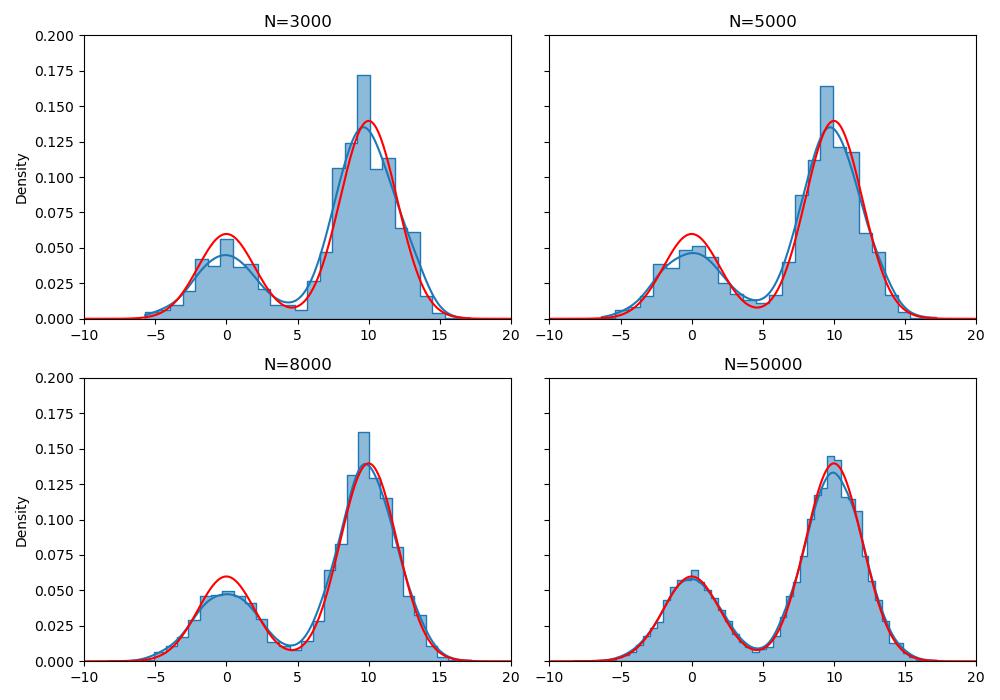
What we can notice is, that the more we sample, the better we match the target distribution. But even for a little amount of samples we get a relativly good match. Further more, we have a pretty high rejection rate. For the last test with 50000 samples only 18171 samples are being accepted. This is pretty bad for us, since it means, we just wasted over 60% of our computing power to produce samples, that we discard.

4 Summary

In this article we took the jump from general independent sampling to MCMC sampling. For this we began introducing some general ideas about Markov Chains and then the Metropolis Hastings algorith,. In the implementation we got a better feeling for how it works in practice and identified the biggest issue, that we will never be sure, if we ran for long enough. With this, the approach has shown to be simple and effective, even though it is not very efficient. In the next article we will talk about Gibbs Sampling, which will be completly parameter free.