1. Introduction to Rejection Sampling

When dealing with complex probability distributions \(p(z)\), direct sampling can be difficult or even impossible. This is where we can use Rejection Sampling, which allows us to sample from a complex distribution with the aid of a proposal distribution, that we can evaluate.

Rejection sampling is especially useful in Bayesian inference when dealing with non-standard distributions that don’t have a straightforward method for drawing samples. In this post, we’ll explore the concept of rejection sampling.

2. Why Rejection Sampling?

Rejection sampling is used when:

• Direct Sampling is Difficult: When we can’t easily sample from the target distribution, rejection sampling provides an alternative method.

• Target Distribution is Known Up to a Constant: To perform rejection sampling, we need to be able to evaluate the target distribution to some normalization factor \(Z_p\) \(p(z) = \frac{1}{Z_p}\tilde{p}(z)\) Preferably with very little effort.

3. How Rejection Sampling Works

The idea of rejection sampling is to sample from a proposal distribution and then “reject” or “accept” samples based on how likely they are under the target distribution.

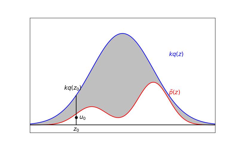
Let’s break it down into simple steps:

1. Choose a Proposal Distribution: Select a proposal distribution \(q(z)\) that is easy to sample from and that roughly covers the shape of the target distribution \(\tilde{p}(z)\). The proposal distribution should be scaled by a constant \(k\), such that \(\forall z: kq(x) \geq \tilde{p}(z)\).

2. Generate a Sample: Draw a sample \(z\) from the proposal distribution \(q(z)\).

3. Generate a Uniform Random Variable: Draw a uniform random variable \(u\) from \(\operatorname{Uniform}(0,1)\).

4. Acceptance Criterion: Accept the sample \(z\) if \(u\leq\frac{\tilde{p}(z)}{kq(z)}\)​. If not, reject the sample and go back to step 2.

5. Repeat: Continue the process until you have enough accepted samples.

The accepted samples will be approximately distributed according to the target distribution \(p(x)\).

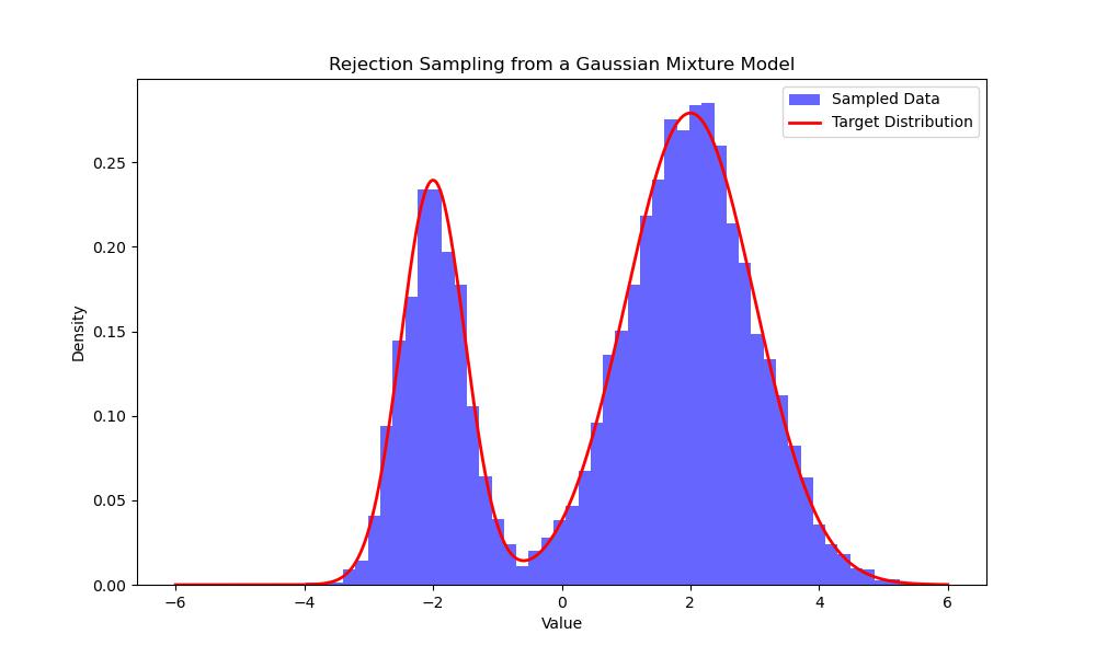
4. Example: Rejection Sampling from a Gaussian Mixture Model

Let’s now consider an example where we want to sample from a Gaussian Mixture Model (GMM), which is a combination of multiple Gaussian distributions as a demonstration.

We’ll use a simple GMM composed of two Gaussian distributions.

The target distribution \(p(x)\) is a mixture of two Gaussian distributions: \(p(x)=0.3\cdot \mathcal{N}(x;−2,0.5^2)+0.7\cdot \mathcal{N}(x;2,1^2)\)

The normalization factor \(Z_p\) in this case is 1, since we can evaluate this function precisly.

We will use a simple normal distribution as the proposal distribution \(q(x)\).

1. Python Code Example: Rejection Sampling

1
2
3
4
5
6
7
8
9
10
11
12
13
14
15
16
17
18
19
20
21
22
23
24
25
26
27
28
29
30
31
32
33
34
35
36
37
38
39
40
41
42
import numpy as np
import matplotlib.pyplot as plt
from scipy.stats import norm

# Define the target distribution (Gaussian Mixture Model)
def target_distribution(x):
    return 0.3 * norm.pdf(x, -2, 0.5) + 0.7 * norm.pdf(x, 2, 1.0)

# Define the proposal distribution (Normal distribution)
proposal_distribution = norm(0, 3)  # Mean 0, std 3

# Define the constant M such that M * proposal_distribution >= target_distribution
M = 1.5  # Chosen to ensure the proposal upper-bounds the target

# Number of samples
n_samples = 10000

# Rejection Sampling
samples = []
while len(samples) < n_samples:
    x = proposal_distribution.rvs()  # Sample from proposal distribution
    u = np.random.uniform(0, 1)  # Uniform random variable

    # Accept or reject the sample
    if u <= target_distribution(x) / (M * proposal_distribution.pdf(x)):
        samples.append(x)

# Convert to numpy array for easier handling
samples = np.array(samples)

# Plot the histogram of the samples
plt.figure(figsize=(10, 6))
plt.hist(samples, bins=50, density=True, alpha=0.6, color='b', label="Sampled Data")

# Overlay the target distribution
x = np.linspace(-6, 6, 1000)
plt.plot(x, target_distribution(x), 'r', linewidth=2, label="Target Distribution")
plt.title("Rejection Sampling from a Gaussian Mixture Model")
plt.xlabel("Value")
plt.ylabel("Density")
plt.legend()
plt.show()

5. Limitations of Rejection Sampling

Now that we gained a rough understanding of how rejection sampling works, we can see that it can be very usefull, but there are also some obvious limitations:

• Efficiency: Rejection sampling can be inefficient if the proposal distribution doesn’t closely match the target distribution. The more samples we reject, the longer it takes to generate enough accepted samples.
• Parameters: Rejection Sampling cannot be simply used. For every usecase we need to find a good matching proposal distribution, which in itself can be very challenging or risk loosing alot of efficiency.
• Dimensionality: In high-dimensional spaces, finding a suitable proposal distribution that covers the target distribution well can be even more challenging, leading to high rejection rates.

Conclusion and What’s Next

In this post, we’ve introduced the concept of rejection sampling, a versatile technique for sampling from complex distributions. We implemented rejection sampling in Python and visualized how the method works in practice. Rejection sampling is a powerful tool but comes with trade-offs in terms of efficiency and complexity.

In the next post, we’ll explore Importance Sampling, a related method that improves efficiency by weighting samples from the proposal distribution instead of rejecting them.